
Here's how this is gonna go, I will not assume that the star is unaffected by the force of other planets and simulate the orbit, only on one planet though, and I will compare that orbit with the orbit we had in the scroll before this one (where my sun is stays at rest). After that, as if all of this wasn't enough, I'll evaluate the accuracy using an analytical approach in that specific orbit.
There are some changes we have to account for first. What is a key characteristic of a suitable frame of reference? It has to be non-accelerating or at rest. Introducing acceleration on the sun, we can't assume that the sun itself won't be moving which means we can't use it as a frame of reference as we have done earlier, now it got a tiny bit more complicated. But fear not my child, it's not difficult. All we have to do is switch the frame of reference to something that will not be accelerating, what could that be, do you have any guesses? It is the frame of reference of the center of mass.
Some boring theory first, I will keep it short I promise! Sir Alfrodius Hafnsen has done most of the work anyway! Here is the derivation of the following.
\(\vec{r}_{1,cm}=-\dfrac{\hat{\mu}}{m_1}\vec{r}\)
\(\vec{r}_{2,cm}=\dfrac{\hat{\mu}}{m_2}\vec{r}\)
Where the reduced mass is given by
\(\hat{\mu}=\dfrac{m_1 m_2}{m_2+m_1}\)
In our last numerical orbit, we found r vector, so what we have to do to adjust our simulator is just multiply it with a constant.
Now when Hafnsen derived them he used that the center of mass is at 0, we will make the approximation that our center of mass is located at 0, the center of mass in our case is (0.00000388,0.00000), so it's a safe assumption to make. So we will use the expressions above. Albeit we do lose some accuracy, otherwise we would use the same expressions for \(\vec{r}_{1,cm}\) and \(\vec{r}_{2,cm}\) but we need to add a constant B which is the position of the center of mass, so it would look like this
\(\vec{r}_{2,cm}=\dfrac{\hat{\mu}}{m_2}\vec{r}+B\)
I will choose the planet I'm on right now. Boring I know, but I chose it because it's close to my sun and not too small for an exaggerated effect. Using the same simulator I used in the last scroll (link), all I have to do is calculate the acceleration for both the planet and the sun, and multiply the results with the appropriate constant, for example for the position of the sun we just multiply with \(\frac{\hat{\mu}}{m_2}\).
Excited to see the results? Me too! Here goes:
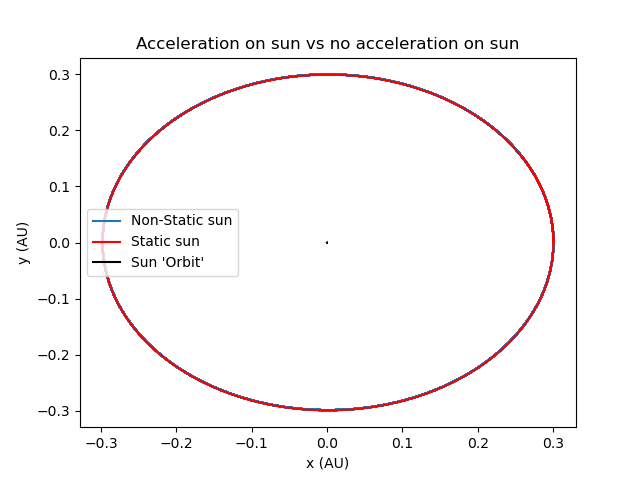
Literally no difference as far as I can see, and you didn't believe me eh? Still some tests to run. The Physica Deorum have taught me the following expressions themselves, these are a 100% true.
E is the total energy of the two-body system:
\(E = \dfrac{1}{2} \hat{u} v^2 - \dfrac{G M \hat{u}} {r}\)
Where \(v= |\dot { \textbf {r} }|\) is the relative speed, \(r = |\textbf { r }|\) is the relative distance, and \(\hat { \mu }\) is the reduced mass and \(M\) is the total mass of the system.
and the angular momentum of the two-body system P:
\(\textbf {P} =\textbf{r} \times \hat{ \mu} \dot{r}\)
Now what would you think these two expressions describe, if you were given no other information other than the expressions (you also don't know what mu is)? To me this looks a lot like a system of one body and what we're trying to do here is make a complex multiple body problem into a single problem by manipulating and introducing constants. This is what we do in physics, break down a complex problem into small constituents that we know how to solve from before.
But given an equation for the total energy is great because we can used it to see if our energy is conserved throughout the orbit, that seals whether this orbit is good enough. If E stays constant we're good alright? WE'RE GOOD.
I will calculate by hand the first 3000 values and see what I get, I will show you the first 10 and the last 10.
First 10
-85.5870962015552
-85.58669623175606
-85.58629997684918
-85.58590744043487
-85.58551862607938
-85.58513353731499
-85.5847521776399
-85.58437455051825
-85.58400065938011
-85.58363050762142
-85.583264098604
Last 10
-86.34696850596
-86.34756812192126
-86.348164155136
-86.34875659958085
-86.3493454492682
-86.34993069824635
-86.35051234059945
-86.35109037044768
-86.35166478194728
This is a good time to introduce the expression for relative error that will be used in further scrolls.
\(\delta = |\dfrac{v_A - v_E}{v_E}| \cdot 100 \%\)
where \(v_A\) is the actual value observed and \(v_E\) the expected value. In our case the first value is the expected value if energy is conserved. Inserting in this equation we get 0.893% relative error, this is quire accurate considering that it's a numerical orbit. A lot of the error comes from the program approximating numbers because it can't represent all the decimals after the digit, so over large iterations we get some error. I believe that energy is conserved to a reasonable degree.
All in all, our model seems to be solid as hell.
Ah according to my calculations a storm is about to set in, I don't have much time to finish writing the next scroll before the storm sets in, storms here last a long time and I'll lose my work, I have to hurry. Next scroll might be my last.