
Okay a lot of stuff will be coming your way but hold tight yeah? It's a mouthful. Let's start off with the one least physics-y, image analysis. I'm just gonna say it, I don't enjoy it but it's a necessary "evil", as Sire Alfrodius used to say
In astrophysics, you need to know a little bit of everything
in order to do a little bit of anything. -Alfrodius Hafnsen
Finding where we're pointing
It is really really important that you understood the scroll right before this one, if you're not feeling 100% go back and take a look at it.
To test whether our technical skill is sufficient, we will attempt to generate a flat picture from a part of the spherical picture, sounds easier said than done. We have a reference picture which happens to be the correct projection, that is, if we generate a picture that is identical to the sample/reference picture, our technical skill is there.
Here is what the sample picture looks like:
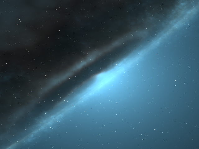
Pretty sky. Let's break the challenge into smaller manageable challenges.
- Find the size of the picture in pixels and the range of (X,Y)
- Generate a (X,Y) grid and thereafter generate the corresponding \((\theta,\phi)\)
- Using the coordinate grids, find the sky image pixel and the corresponding RGB colors.
Okay 1st challenge is easy, all we have to do is use the PIL module which helps us open and manipulate PNG files, from there we import the image and use the numpy library to put the picture in array form which has the shape (y-pixels, x-pixels, 3), finding the y and x pixels was the goal here. I did this and got y-pixels 480, x-pixels 640, so the resolution is 640x480, which makes sense because the picture is wider than it is tall. Given those pixels, we can find the range which for the x-pixels is just \(X_{\text{max,min}} = \pm \dfrac{\text{total x-pixles}}{2}\), the same follows for Y. From this we get, X = (-320,320) and Y = (-240,240)
Second challenge To make coordinate grids, this is very easy using numpy libraries but the idea is to make a meshgrid. If you have your math book has these squared boxes on the paper then that's basically a meshgrid, every point where one line crosses another has a value of x,y. I don't want to go in depth here, but if you would like to check this video out. So we basically make an equally spaced grid with the limits we established already in the last challenge, such that each step is 1 pixel, this having a grid with each possible pixel.
From there we can iterate over our grid and convert it to a different kind of grid, one that looks like this.
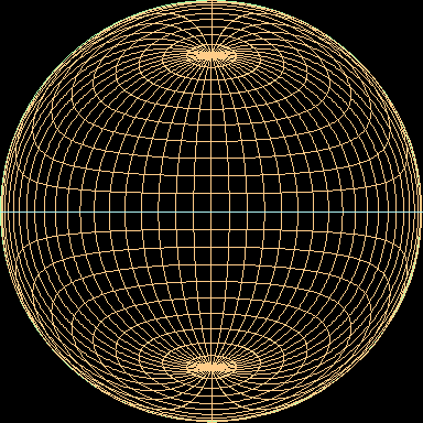
This is a simple task, we only have to calculate:
\(\theta=\theta_{0}-\arcsin\left[\cos\beta\cos\theta_{0}+\dfrac{Y}{\rho}\sin\beta\sin\theta_{0}\right]\)
\(\phi=\phi_{0}+\arctan\left[\dfrac{X\sin \beta }{\rho\sin\theta_0\cos\beta-Y\cos\theta_0\sin\beta}\right]\)
Where:
\(\dfrac{2}{\kappa}=1+\cos\theta_{0}\cos\theta+\sin\theta_{0}\sin\theta\cos(\phi-\phi_{0})\)
\(\rho=\sqrt{X^{2}+Y^{2}}\)
\(\beta=2\arctan\dfrac{\rho}{2}\)
Now that we have a spherical grid we're ready for the next challenge.
Third challenge We have a 360 picture of the night sky from a wonderful satellite orbiting right now, in a numpy array named himmelkule.npy, which has for each spherical coordinate a unique pixel index for each 3 numbers that tell us the color of that specific pixel, the 3 numbers are RGB values. The gods have gifted us a function that finds the index of the pixel in the full-sky image (himmelkule.npy) corresponding to the given spherical coordinates. Using the 360 picture, the function gifted to us and our grid generated from last challenge we can try to generate our very own image.
The way to do is to iterate over each x-pixel and all y-pixels (a nested for-loop if you're familiar), and find the special index using the gifted function, we insert that special index and find the RGB values, then we fill an empty array with shape (480,640,3) with the RGB values obtained, we save the image and get disappointed more often than not. It can be hard to explain this so I've made an exception this time and I'll include code at the very end just for you to see how things get implemented.
Let's look at the results:
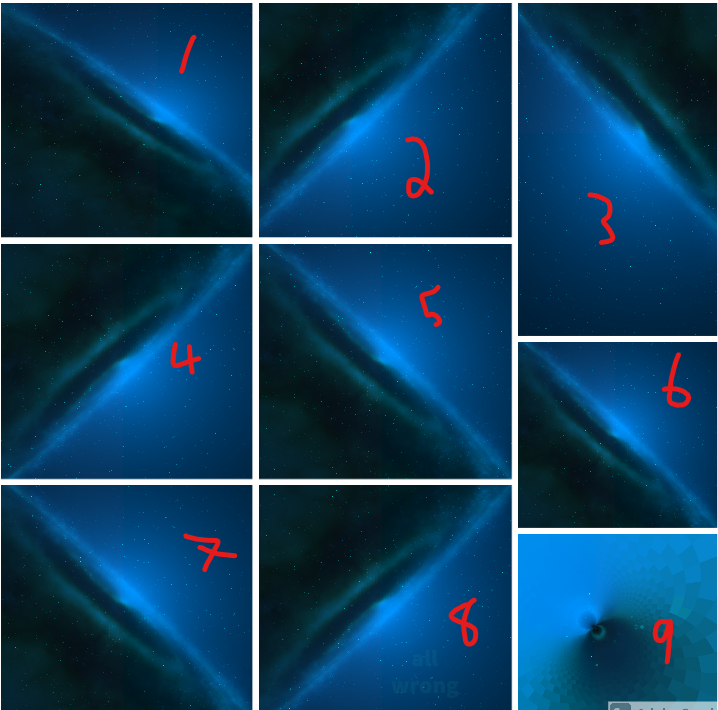
You can see how massive a failure some of these are, but that's just the way it is, one thing i realized is that the color is off, and that picture number 8 is correct but has wrong RGB values. I tried to fix the RGB values by changing the indexing and so on, here's what I got:

Now the color is correct, but the image is not exactly identical. Upon closer analysis we see that the image starts out (bottom left corner where we start the index) correct and the farther away it goes (to the top right) the worse it gets, so it's got something to do with the iteration, perhaps some values are being indexed too soon. I tried a lot to find what the issue was but I've ran out of ideas so it will have to suffice, and it will in fact suffice, here's why.
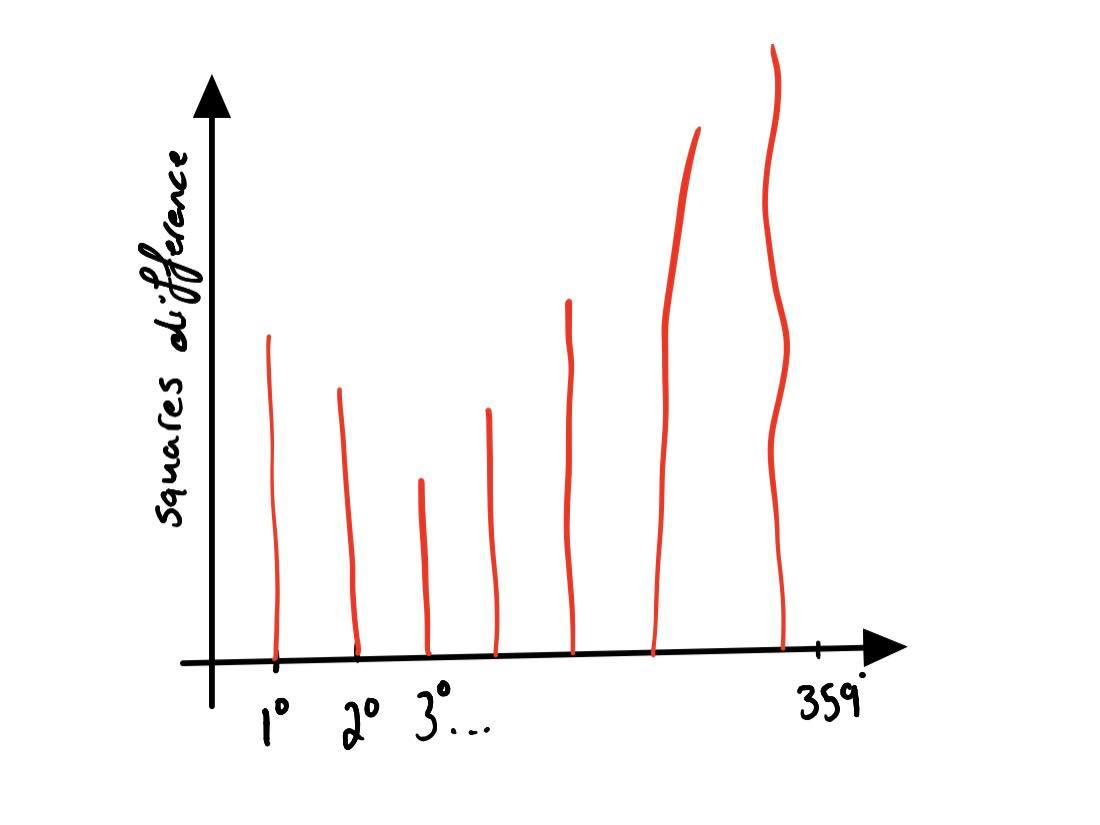
Perhaps explaining this earlier would've been a better choice but the reason we're doing this is so that when we take a picture using our spacecraft, we'll compare that picture with the night sky which we assume stays still, we can generate stereographic images for each angle (0 deg to 359 deg) and save them somewhere. So in a nutshell, find out which image (0 deg ... 359 deg) looks most similar (RGB values align) to the image we took from the camera, this way we get to know at what angle we're pointing thus finding out where we're looking which was the whole point.
The actual method to doing this would be the least squares method, taking the difference between our RGB values at each pixel and RGB values for each image (by iterating) squared, then we plot that and get a graph that can look something like this:
Finding our Velocity
Here’s a short introduction of how we’ll find our velocity with respect to the sun. We’ll use two reference stars, measure their wavelengths, and use that to find our own velocity.
How do we find our velocity:
We’ll break the problem down into smaller doable challenges.
- Find a formula that determines radial velocity with respect to the stars and find the radial velocity of the sun with respect to the stars
- Investigate the special case scenario where \(\Delta\lambda\) is measure to be 0 by the spectrograph on our spacecraft, what is the velocity with respect to the reference stars? What is the velocity of the craft with respect to the sun?
- Transform the velocity to x,y velocity where the sun is at origin
Knowing \(\lambda_0\) (656.3 nm) and c as constants, we see that the radial velocity is dependent on the observed wavelength, so we basically have radial velocity as a function of observed wavelength. Through observations done many years ago, I know that \(\Delta\lambda\) at the sun are:
(-0.001846798631072184, -0.015944684555921993)
From this we can obtain the velocity of the sun with respect to each star
Star 1:
\(v_r =\dfrac{\Delta \lambda_1}{\lambda_0}\cdot c\) We don't change units from nm to m because they cancel out anyway.
Star 2:
\(v_r =\dfrac{\Delta \lambda_2}{\lambda_0}\cdot c\)
You might be wondering why is finding the radial velocity of the sun with respect to the stars of any help, the reason is the frame of reference can help us find the velocity of our spacecraft with respect to the sun, here’s how. Let’s say you’re watching 2 runners moving at constant velocity, runner A has velocity 5 m/s and runner B has velocity 8 m/s with in your frame og reference. The question is, can you find the velocity of runner B with respect to runner A? If you can’t see it yet, think that you are runner B and you’re looking to your left where runner B is running, how would his velocity seem? He’s moving faster than you are but just by 3 m/s, so that’s what you will see. To guide your intuition further, think of when you’re in a car and the car driving right next to you with same velocity seems like it’s not moving at all with respect to you, if a car is a bit faster than you at let’s say 100 km/h and you drive at 95 km/h, the car won’t zoom past you are 100, it will move ahead of you at 5 km/h.
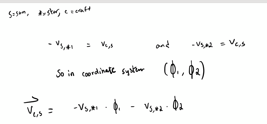
So we’ll be doing the exact same but instead of two cars/runners and an observer, we have the sun and you, and the reference star as the observer. So if we have the radial velocity of the sun with respect to each star, and the radial velocity of our spacecraft with respect to each star, we can then subtract the sun’s velocity from the spacecraft’s velocity and we get the spacecraft’s velocity with respect to the sun, in \((\phi_1,\phi_2)\)coordinates. In other words (or should I say signs)
\(v_{\text{c,*}}-v_{\text{s,*}}=v_{\text{c,s}}\)
where \(v_{\text{c,*}}\) tells us the velocity of the c (spacecraft) with respect to * (the star)
Okay let’s get back to solving the problem:
In the case where \(\Delta\lambda=0\) we get: \(0-v_{\text{s,*}}=v_{\text{c,s}}\) because if the change in wavelength is 0 then there is no radial velocity.
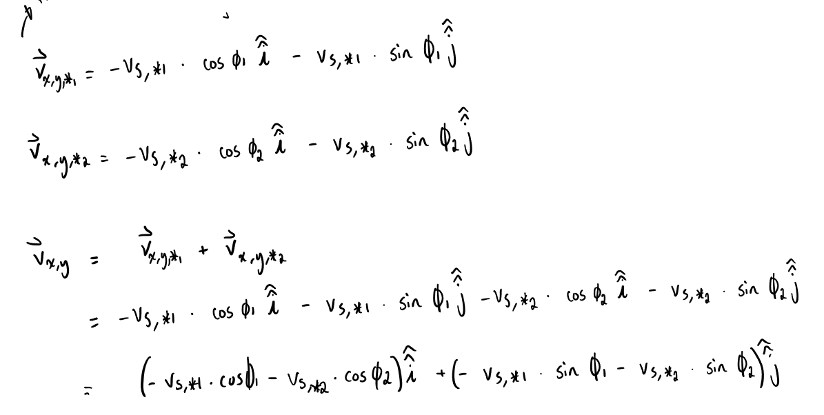
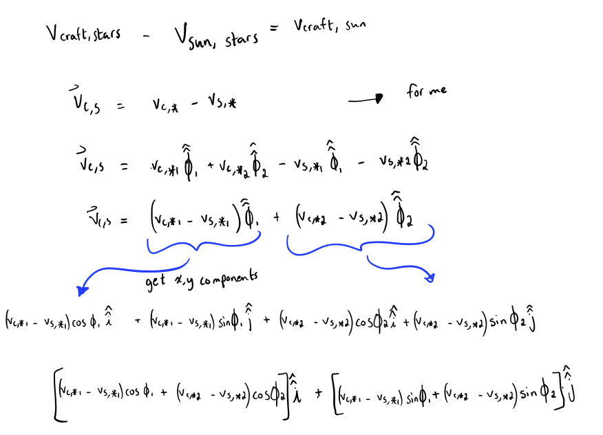
But to convert the velocity into x,y we use trigonometry, the following diagram should aid your understanding. If we decompose each of the velocities into x,y and then add up the x and y components we can find the velocity in the xy direction.
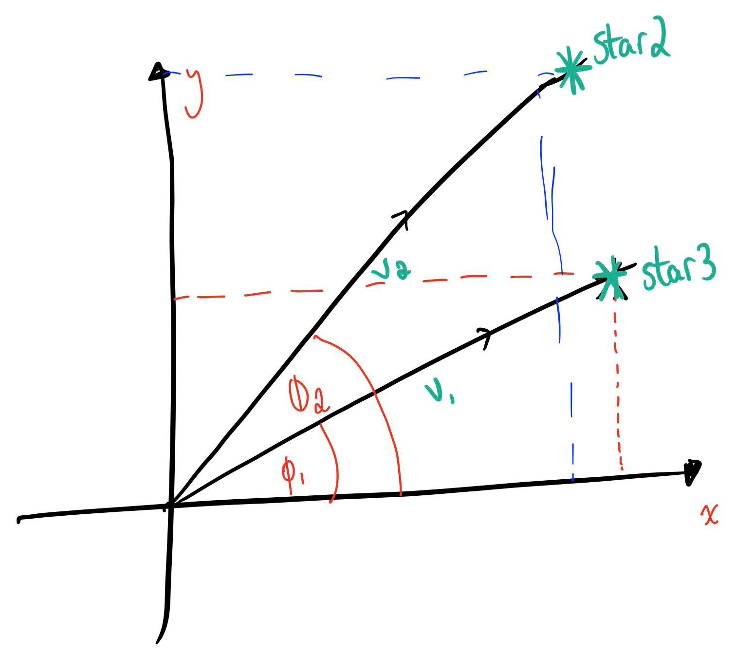
I was unsure whether I should show you the math to derive the equations but hear me out, I'll put it out there, just look past the next images alright? If you don't understand it 100% it's not your fault, I'm not exactly the best at written mathematics and I also wrote very little explanation.
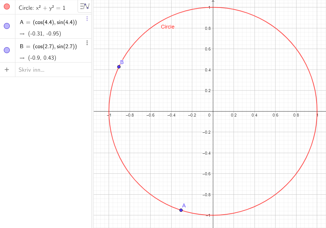
Inserting the values, where \((\phi_1,\phi_2)\) is \((4.44,2.73)\) approximately, and \(v_{\text{s,*1}}=-843.6, \ v_{\text{s,*2}}=-7283.4 \), inserting for these values we get that the velocity of the spacecraft with respect to the sun is \((-6921.69,2048.3)\) respectively. Let's try to see if it makes sense, here are the angles on a unit circle to give us an idea of the angle at which the stars are located, we also see that the velocity is much higher in the direction of the second star (star B) so the final velocity we get makes sense, given that the velocity is in the negative x direction and positive y direction.
Now is time to test out our model but more generally, as we usually do, we have two situations, delta(lambda) = 0 and when the craft is on the surface of the sun (realistic I know), if we get values that make sense then we can assume it works, now we have to do the math allover again, I'll attach the images but just skip over it if it's not your thing
Ah, the scroll got ripped to shreds from the wind, I will have to rewrite what I had already lost, how frustrating it is when your work isn't saved. Now the only difference from our previous equations is the velocity measured using the values obtained from the spectrograph on board the ship.
We will examine this equation by running it through two scenarios, the spacecraft being on the surface of the sun and the spacecraft having delta(lambda) = 0. If the spacecraft is on the surface of the sun then the delta(lambda) is equal for both of them, inserting that into our equations we get (0,0), no surprise tho, we are literally on the surface of the sun that's stationary.
The other test is not exactly bulletproof but we just want to se if the technical stuff is working, we try delta(lambda)= 0 and we got the expected value. Now listen, I did good and all but I feel something's off, like I'm missing something, like the test should be more rigorous and my method is not, however, sometimes you just gotta do the best you can son and let it go.
Finding our Position
I'll make this concise, short and sweet, you've been through enough gibberish already. Our spacecraft is equipped with radar arrays that are able to find the distance between us and other astronomical bodies, and we want to find our position with respect to the sun. So what do we do?
Well first let's think about how many measurements (distance to how many bodies) do we need? Take a guess, we'll find out in a moment. Let's start from 1 measurement, well now we know that we are at a distance 1 AU from a planet, does that pinpoint where we are? Not exactly. There is a whole circle around that planet with radius 1 AU that we could be at.
Okay maybe 2 planets, let's try it out.
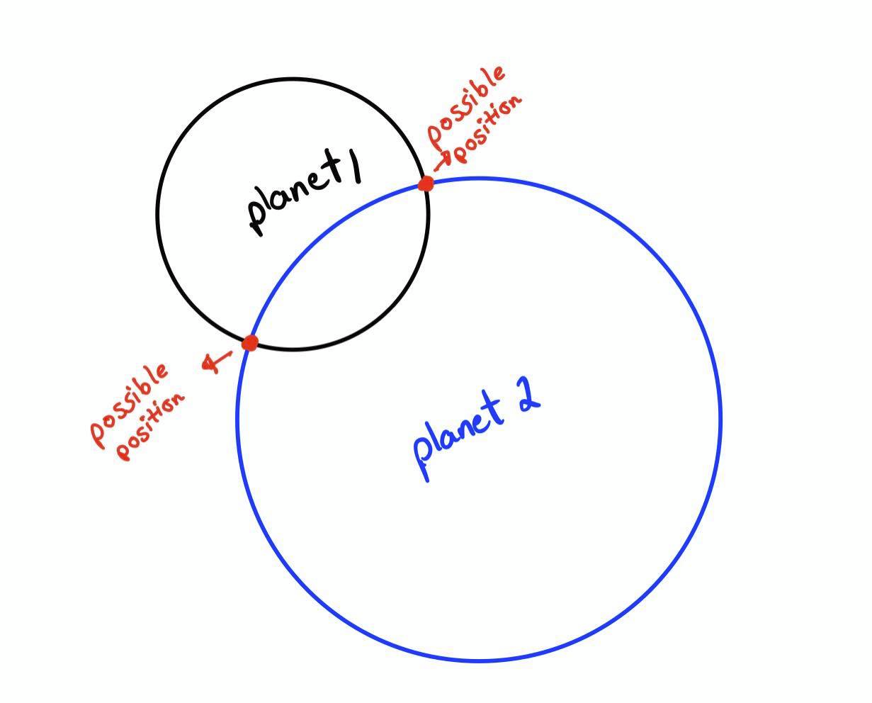
Alright as you can see there are two positions, but we're definitely getting closer. Here's what 3 measurements looks like
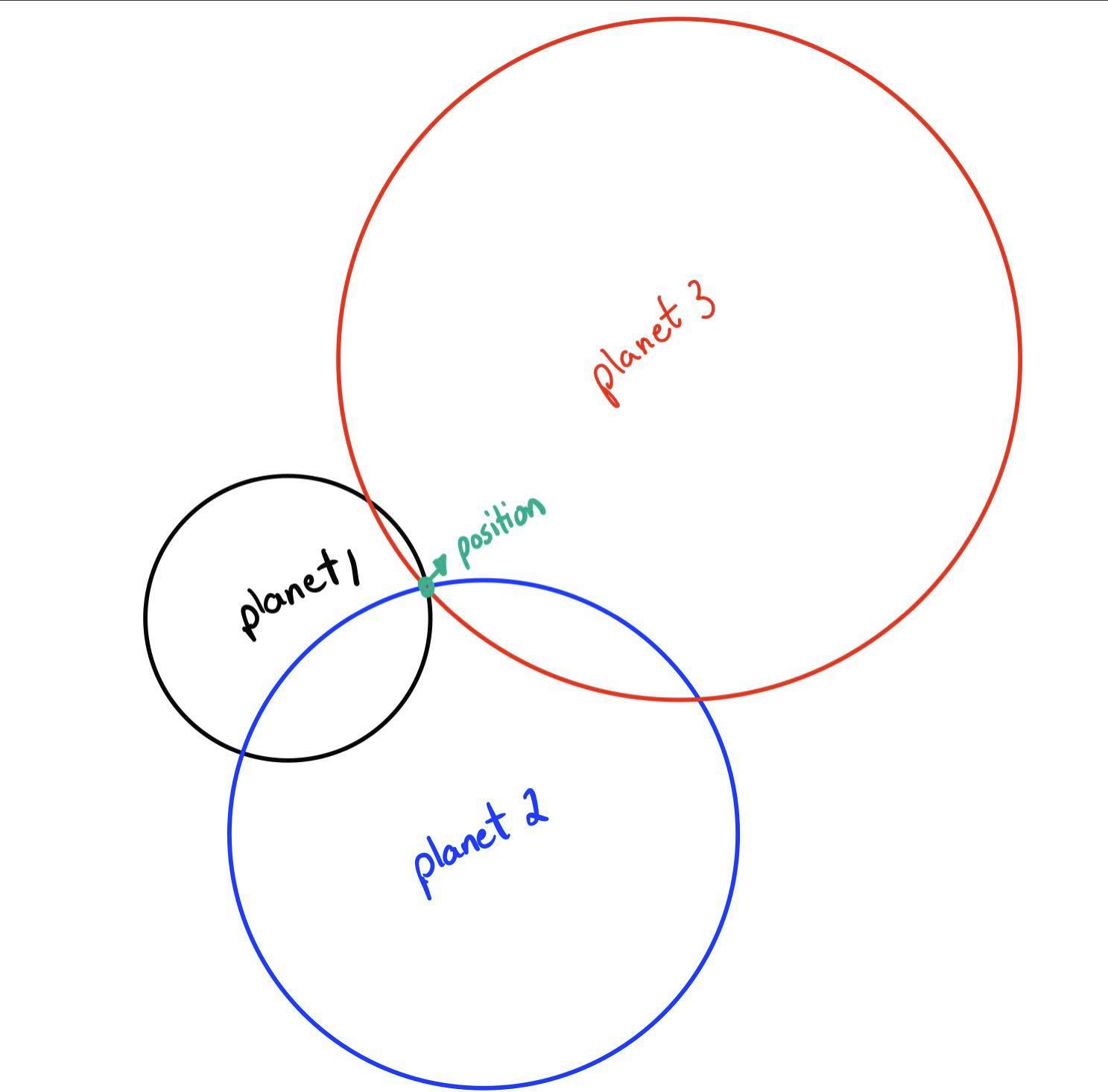
Eyy now we can pinpoint our location! Or can we? Well it's actually more simple than you think, we know the position of each of our planets in the x,y axis centered at the sun from previous scrolls, and we also know the distance but we know that each and every circle here satisfies the equation of a circle which is as follows
\((x-x_0)^2+(y-y_0)^2=r^2\) Where \(x_0,y_0\) is the position of the center of that circle, do you see that we have all we need? We have 3 equations, one for each circle we have from the figure above, if we set up a system of equations we can quite easily solve them. So we basically set up equations as such
\((x-x_1)^2+(y-y_1)^2=r^2_1\)
\((x-x_2)^2+(y-y_2)^2=r^2_2\)
\((x-x_3)^2+(y-y_3)^2=r^2_3\)
Solving for x,y gives us the values we're looking for.
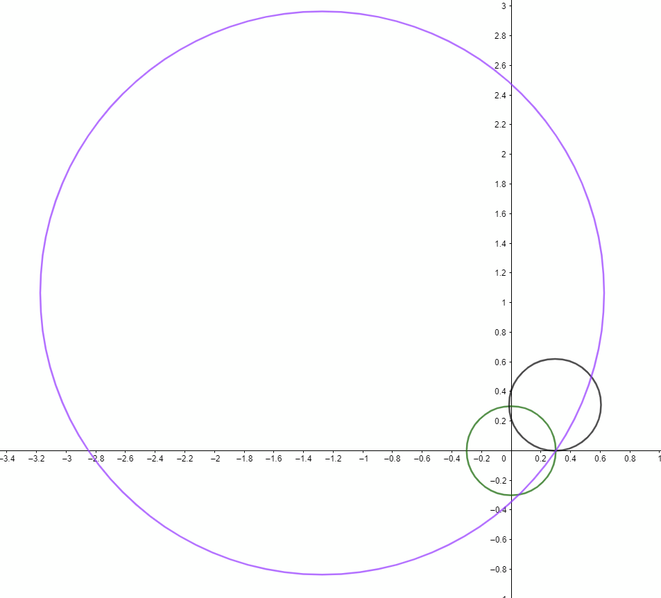
We test our model by pretending we're on the surface of my planet at time 0, where planet 1 is 0.309 AU far away, at position (0.295,0.309) and planet 2 is 1.900 AU far away, at position (-1.274,1.064) and the sun at position (0,0) at distance 0.3005. Using these measurements and solving for x,y we get 0.3005 AU which is exactly what we were expecting. Here is a figure showing the system, y axis and x axis is position in AU, I used the software Geogebra to make this drawing using just the equations above with known values inserted. It really was that simple.
OOOOOOKAY finally we're done with the challenges. Time to recap and discuss. We wanted to navigate space so we agreed that the most important things we need is know is our position, velocity and where we're pointed (angularly speaking). We found where we're pointed by taking a picture and comparing it to the reference 360 pictures, and finding the least difference, 360 pictures with one degree between them is not too much but it enough given that we're going to gigantic planets. We also found out our velocity using the doppler shift data measured on board the craft and the doppler shift data measured on the sun. The position which was relatively simple, was just solving a system of equations using 3 bodies. We tried to test out our data and methods and got the results we expected.
How could we have had more accurate results? Well the only thing would be to have more angles instead of just 360, perhaps 720 from 0 to 359, we would then get slightly more accurate directions. Otherwise, it's all up to the machinery and how accurate the measurements are. I would like to add that our results are realistic because the tests we did gave us good results. Well that concludes our mission for this time. We'll meet again next time.
Where:
Figure 1: https://subscription.packtpub.com/book/big-data-and-business-intelligence/9781786463517/6/ch06lvl1sec51/meshgrid-and-contours