
You're on a ship in the 1800's, you're the captain of that ship in fact. What are the most important things you need to know to be able to navigate the mighty oceans? Well, I would nominate these:
- You need to know where your ship is headed (direction)
- You need to know where you are (position)
- You need to know how fast you are sailing (velocity)
.jpg)
I have to force myself to not talk about ship navigation because I would go on for days on end, but if you're interested in the history of navigation check this book out. Well we're also going to be launching ourselves in uncharted territory and we need some navigation tools, and it turns out we need the exact same things to be able to go around. I mean outer space is not all that different from navigating uncharted maritime territories, except if you mess up a bit on your spacecraft it will most likely be the last mistake you'll ever make.
In this part you will be familiar with some core concepts of velocity and all that jazz but the method at which we'll arrive at it is a bit funky to say the least.
This scroll will introduce and explain all the theory and toolkits needed to tackle the navigation problem.
Spherical coordinate system
Remember the polar coordinate system? This one is pretty much identical except we add a new angle called the azimuthal angle \(\phi\). I strongly recommend you go refresh your memory on the polar coordinate system, here.
A good figure is worth a thousand equations
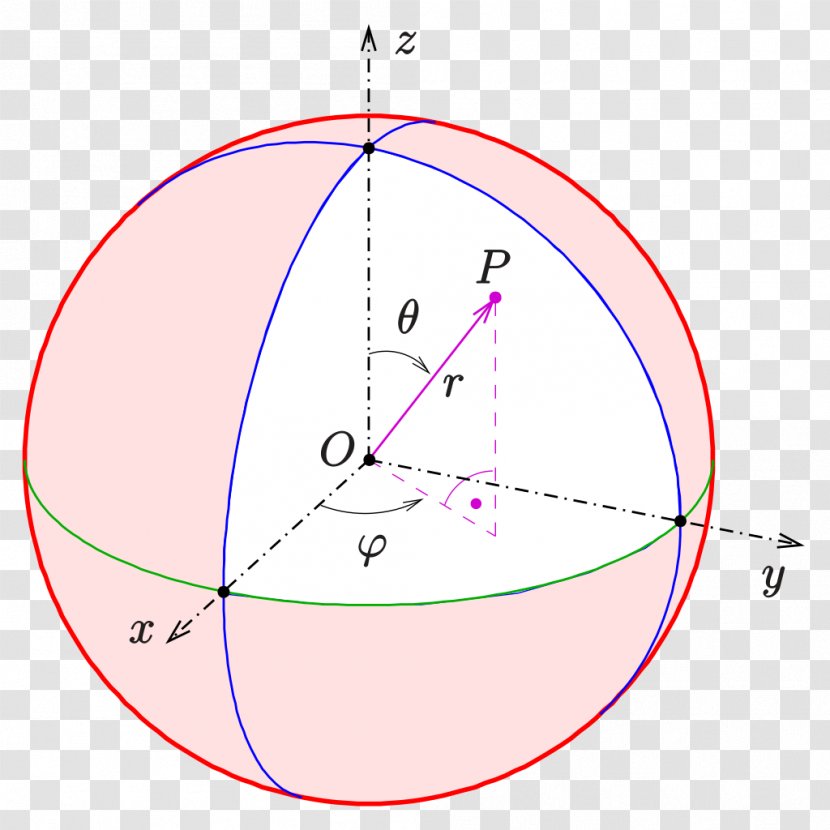
Notice that if we remove the z axis, we just get polar coordinate system, so the function of that extra angle is to make polar coordinates from 2D into 3D. Explaining this coordinate system is a bit futile but the best way to learn it is to experiment with it, try to pinpoint a random point on that sphere and try to see for yourself that the coordinate system we have can pull it off.
Note that we chose the azimuthal angle to be phi but in other textbooks and classes it's swapped with theta.
Stereographic Projection
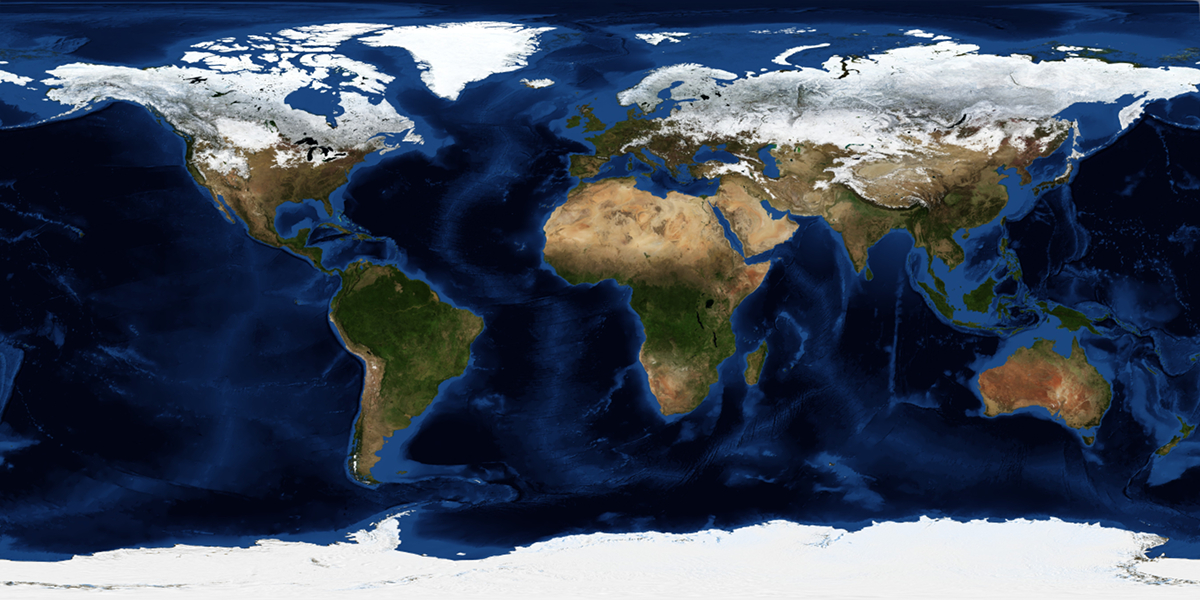
Pretty standard map right? We take flat maps for granted but we kind of shouldn't, here's why: Earth is a sphere, how can we project a sphere onto a piece of flat paper, try to picture it. You can't do it without sacrificing some accuracy.
Here is a figure showing how the projection works.
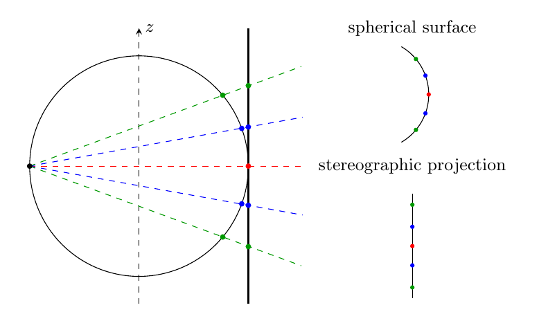
It's a bit subtle but look at how the distance between the red dot and the blue dots is smaller than the green dot and the blue dot. You might think this is a good enough approximation but I would beg to differ. Here is a consequence of this projection: Greenland
.jpg)
It's true, greenland looks almost the size of all of Africa but if we had projected it on the equator it looks much much smaller, makes you wonder how many other countries look huge because they're far down or up.
We must be able to switch back and forth from stereographic projection to a surface-view. Here's a figure demonstrating a 3D version of stereographic projections
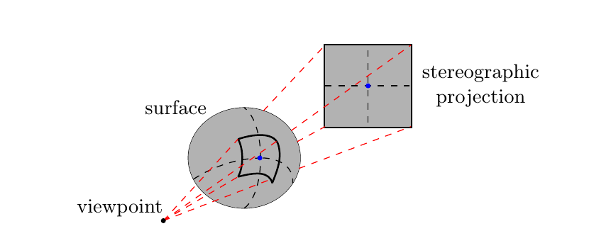
As usual, I present the resulting expressions and link to the tedious derivation for those who are interested in deriving ugly equations. Here are the results.
\(X=\kappa\sin\theta\sin(\phi-\phi_{0})\)
\(Y=\kappa\left(\sin\theta_{0}\cos\theta-\cos\theta_{0}\sin\theta\cos(\phi-\phi_{0})\right)\)
\(\theta=\theta_{0}-\arcsin\left[\cos\beta\cos\theta_{0}+\dfrac{Y}{\rho}\sin\beta\sin\theta_{0}\right]\)
\(\phi=\phi_{0}+\arctan\left[\dfrac{X\sin \beta }{\rho\sin\theta_0\cos\beta-Y\cos\theta_0\sin\beta}\right]\)
Where:
\(\dfrac{2}{\kappa}=1+\cos\theta_{0}\cos\theta+\sin\theta_{0}\sin\theta\cos(\phi-\phi_{0})\)
\(\rho=\sqrt{X^{2}+Y^{2}}\)
\(\beta=2\arctan\dfrac{\rho}{2}\)
Pictures
Let's take stereographic projections a step further and look at pictures. A camera has boundaries on what it can project. We have FOV again which was introduced a few scrolls ago. Let FOV be \(\alpha_\phi \times \alpha_\theta\) where the azimuthal angle is the maximum angular width and the theta angle denoting the maximum angular height. In other words.:
\(\alpha_\theta = \theta_{max}-\theta_{min}\) and \(\alpha_\phi = \phi_{max}-\phi_{min}\)
Using these limitations and the adjustment needed to center the image at a specific theta or phi.
\(-\dfrac {\alpha_\theta}{2} \leq \theta -\theta_0 \leq \dfrac{\alpha_\theta}{2}\) and \(-\dfrac {\alpha_\phi}{2} \leq \phi -\phi_0 \leq \dfrac{\alpha_\phi}{2}\)
We have already established a relationship between the angles and X and Y, so if we set a limitation on the angles we set a limitation on X and Y. Using the relevant equations the limitations look like this:
\(X_{\mathrm{max/min}}=\pm\dfrac{2\sin(\alpha_\phi/2)}{1+\cos(\alpha_\phi/2)}\) and \(Y_{\mathrm{max/min}}=\pm\dfrac{2\sin(\alpha_\theta/2)}{1+\cos(\alpha_\theta/2)}\)
Another expression we'll use is the doppler shift/effect, here it is for repetition.
\(\dfrac{\Delta\lambda}{\lambda_0}=\dfrac{v_r}{c}\)
where \(\Delta\lambda\) is the difference between the observed wavelength and the wavelength seen from the rest frame of the object emitting the wave \(\lambda_0\), in our case we're using a specific spectrum. \(v_r\) is radial velocity and \(c\) is the speed of light, all SI units.
Want to see how this all plays out? Join me here to check the method with which I will use this theory and those equations to find the velocity, direction and the position.
Figure 1: https://sakhalianet.x10.mx/shippictures/art_sailing_frigates.htm
Figure 2: https://en.wikipedia.org/wiki/Spherical_coordinate_system
Figure 5: https://www.geospatialworld.net/blogs/maps-that-show-why-some-countries-are-not-as-big-as-they-look/