
We'll be simulating the spacecraft's trajectory given a few initial conditions: \(t_0,r_0\ \text{and}\ v_0\). We will not be using our mighty engines, we'll just coast freely. What is it that affects our trajectory here? Just the gravitational pull from all the planets. We look first at the gravitational pull from one planet.
\(F = \dfrac{GM_pm}{|\vec r-\vec r_p|^2}\cdot\dfrac{\vec r-\vec r_p}{|\vec r-\vec r_p|}\)
A bit to unpack here. G is the gravitational constant, \(M_p\) is the mass of the planet, m is the mass of the spacecraft, \(\vec r\) is the position vector of the spacecraft with respect to the sun at origin, \(\vec r_p\) is the position vector of the planet with respect to the sun at origin.
The last fraction is what we call the unit vector, that's just a vector that has length 1 which means when you multiply it with a scalar the magnitude doesn't change, just the directions do, so the unit vector just gives us the correct direction. This term \(|\vec r-\vec r_p|^2\) is just the usual R you're used to, except we're finding the vector that's pointing from the planet to the spacecraft then we find the length of the vector.
This is nice and all but we must find the gravitation pull by each and every planet, so we'll need to find the sum of the force by each planet at a variable r then add the pull by the big boss, the sun. Let's write this up in mathematical terms
\(F=-G\dfrac{mM_s}{|\vec r|^3}\vec r-\sum^N_{i=1}\dfrac{GmM_i}{|\vec r-\vec r_i|^3}(\vec r-\vec r_i)\quad (*)\)
where m and \(\vec r\) are the mass and position of the spacecraft, \(M_s\) is the mass of the star \(M_i \ \text{and}\ \vec r_i\) are the mass and the position of the planet \(i\). Now we have what we need.
An illustration of the formula above:
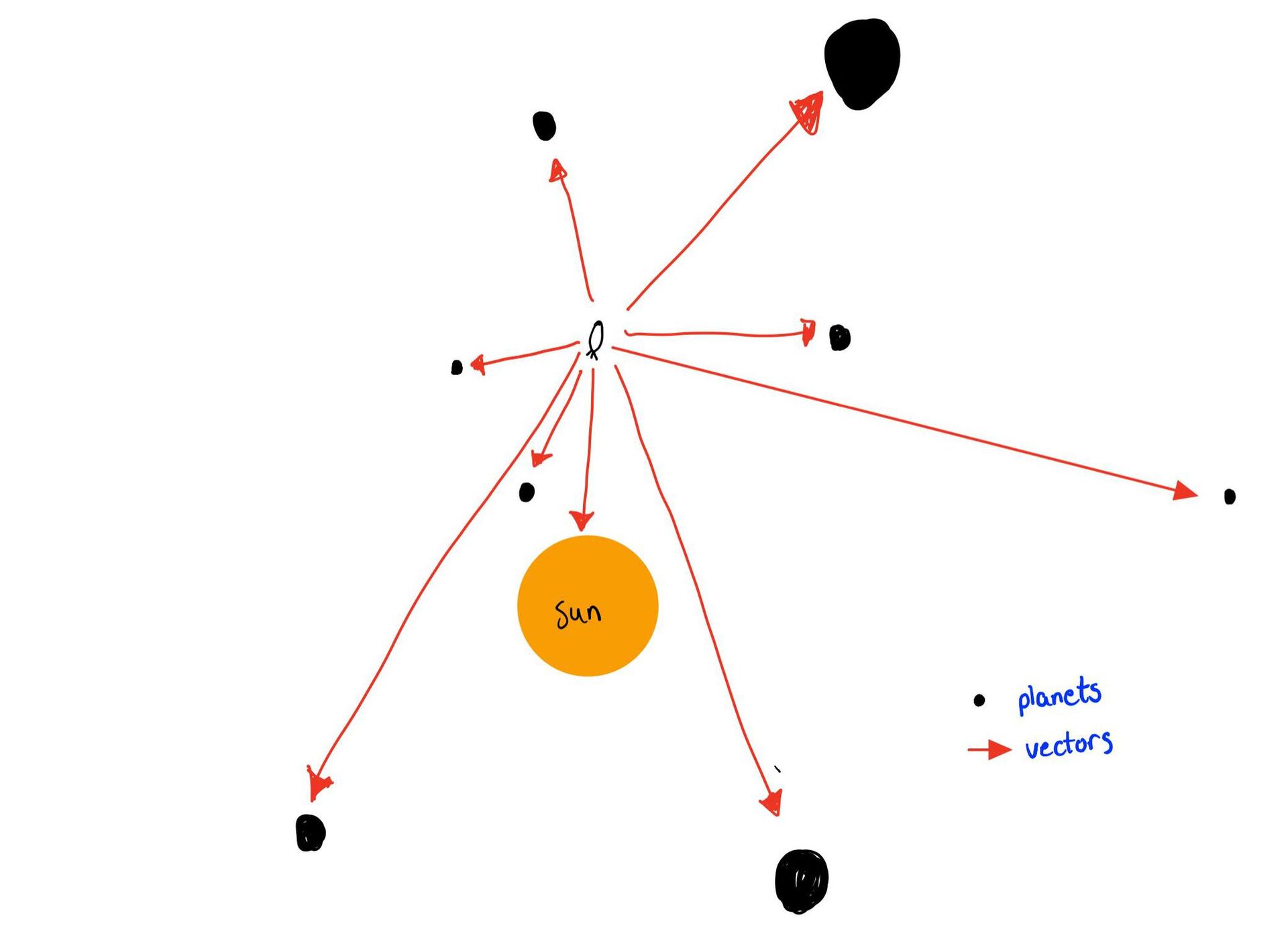
So what we're doing in that formula above is just adding all the red arrows together, that summation sign is a fancy way that saves us time writing the gravitational pull of each and every planet.
In other words, F increases when the body is close and massive, but closeness is a lot more important because the force is inversely proportional to the distance squared. Here are some relevant values:
| Things | Mass (kiloton) |
|---|---|
| Titanic | 52 |
| Planet 0 | 7 767 959 |
| Planet 1 | 1 492 691 |
| Planet 2 | 19 821 |
| Great Pyramid of Giza | 5 216 |
| Planet 3 | 164 285 428 |
| Planet 4 | 407 035 |
| Planet 5 | 827 719 |
| Planet 6 | 586 269 |
| Planet 7 | 9 956 817 |
| Our sun | 600 895 906 968 |
| Your mom | \(\infty\) |
Just joking. I meant the mom's of the gods who exiled me.
Okay but why are we calculating the force? Well we can find the acceleration from the force and from that we can use our favorite integration algorithm to find the velocity and the position which is exactly what we need to find to solve for the trajectory. Remember the leapfrog integration algorithm? That's the one we're using here again, if you forgot please revisit it here. The reason I use this algorithm method is because the speed, simplicity and precision are quite good for my needs and my computer's computing power. On top of that, it conserves energy.
Before we unleash ourselves at the detailed method, we have to understand interpolation which plays an instrumental role here. Previously we found the positions of all the planets and the associated times, but make no mistake, these were just datasets that perhaps looked like this. Note that the numbers are not accurate but rather chosen for pedagogical reasons.
| Planet 0 Position (AU) | At time (yr) |
|---|---|
| (0.3,0) | 0 |
| (0.28,0.12) | 0.1 |
| (0.20,0.9) | 0.2 |
| ... | ... |
What is the position of the planet at 0.15? We don't know exactly, because our data set is not a continuous function. What is the solution? Interpolation. It is the process of estimating unknown values that fall between known values. A diagram to guide your intuition:
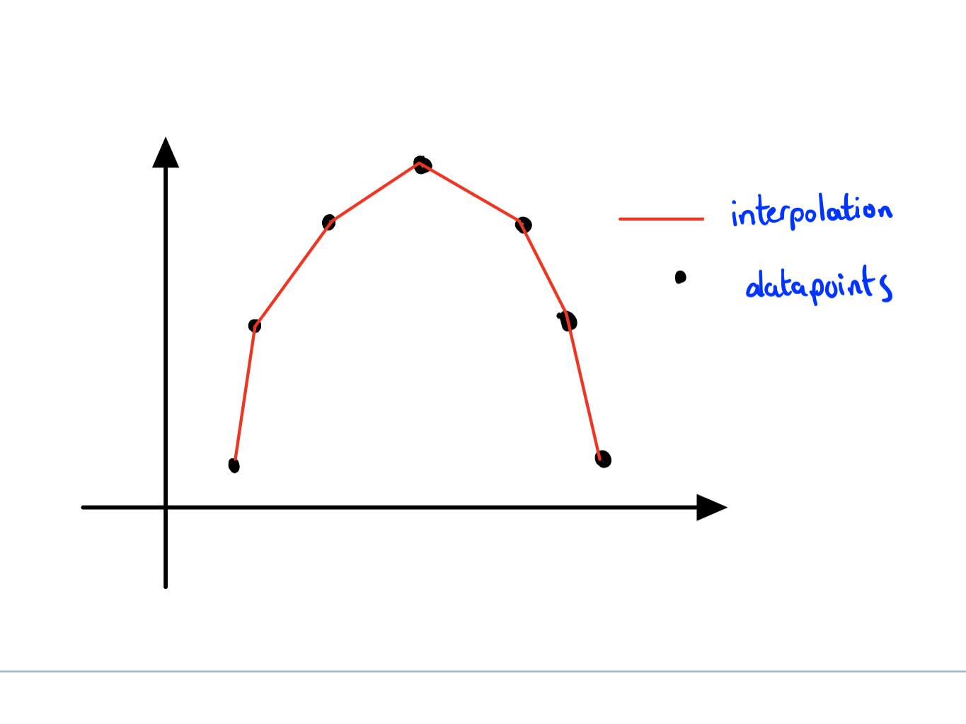
From the figure we can see that perhaps it is a second degree polynomial, but since the positions of the planets are not very easy like this one we have to use the help of SciPy library which can do the interpolation for us, or in other words find us a function that fits it well. Note that in Figure 2, if we increase the number of datapoints or decrease the distance between datapoints we get a finer looking graph and thus a better function. We use SciPy to interpolate the data set we have and thus obtaining a function that returns the positions of all the planets at any t.
What's a good way of implementing a function/algorithm that finds the position? I have a suggestion:
The function receives the necessary variables, the masses of the planets, the total time of the launch, time steps, initial position and initial velocity. Then we have a loop that goes over the number of data points we wish to have and inside that loop we do the following:
- Find the positions of all the planets using the interpolated function
- Find the force by the planets on the spacecraft using formula (*)
- Then we find the acceleration by dividing the force by the mass of the spacecraft
- Having an acceleration function, we use leap frop to obtain/return spacecraft position.
Seems good, I have a good feeling about this, let's test run this. We'll be testing the function by adding a random initial position then setting the initial velocity to be that of the necessary velocity to stay in orbit around the sun using this expression \(v=\sqrt{\dfrac{GM_p}{r}}\) but in vector form.
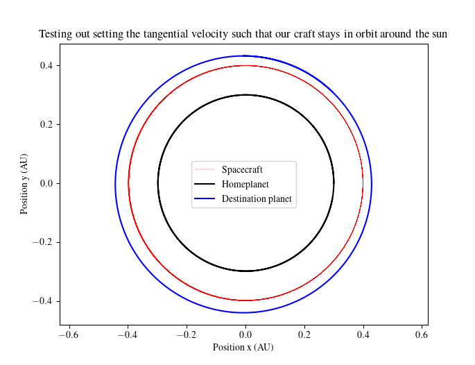
Ey that's pretty good. The red orbit is our spacecraft's, and we see that it is more or less in stable orbit as we expect, given that the velocity at that position is exactly the velocity needed to keep it in orbit. We chose initial position to be (0.4,0.0) AU such that the tangential velocity is just one component, making it a tad bit easier and more fool-proof. One subtle but important observation we make is that on the right side of the orbit it's closer to the blue orbit, that is the destination planet's orbit. There are several reasons that can be the reason, one major reason is that the destination planet is close to the spacecraft at some point which makes the orbit a bit closer, another reason could be that the other planets, especially the massive ones happened to be on that right side, there is more to discuss but this is not the main focus here. Let's look at what happens when we change the velocity by various factors.
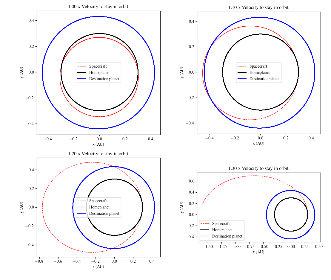
In all of the graphs above the initial position was the same as that of our home planet which is why it is different from the figure right before this one. The first figure we see a normal orbit which is skewed somewhat to the bottom and the reasons for this could be the same as we have explained before for figure 3. In the second figure we see that a factor of 1.10 will launch us to the next orbit which is what we wish to do. In the third graph we see the same thing but instead the ellipse is much larger. In the final graph we have an ellipse even larger.
Say after me: Thank god for Walter Hohmann. This man made analytically transferring from one orbit to another a walk in the park. Let me lay it down on you first then we'll try to apply it and see if we get somewhere. As usual, the math is kept to a minimum but in this document you'll find more information such as the derivation and applications, be sure to check it out for deeper understanding of the Hohmann transfer. Okay let's dive in:
What exactly is a trajectory transfer? It is just changing your orbit to another desired orbit, regardless of higher or lower but in our case we're going higher because planet 1 has an orbit with a large semi major axis. Fuel is not free, and you can only carry so much, thus choosing a minimum energy approach is favorable, and that is exactly what the Hohmann transfer is, a minimum energy transfer, allowing us to carry more equipment and less fuel. This is how NASA sent their Mars InSight probe, check this animation out.
The Hohmann consists of two steps, an impulse, or an instantaneous acceleration at two different positions, that's pretty much it with some other details, but that's the core concept. Let's look at the first step.
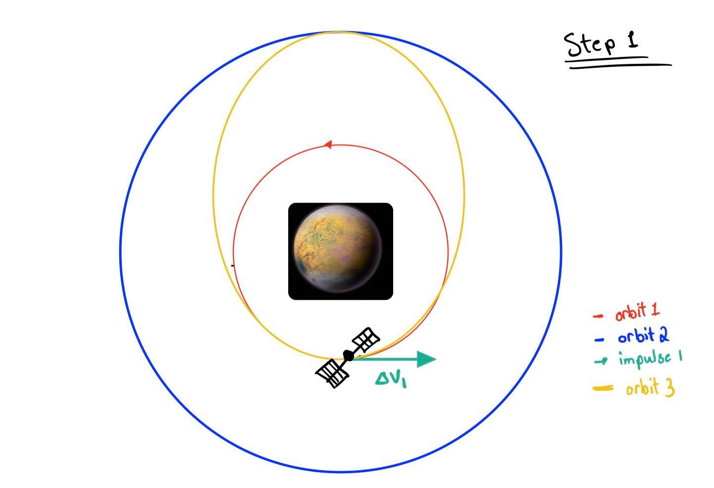
While the satellite is orbiting the sun, it makes boosts equivalent to \(\Delta v_1\) which is given by:
\(\Delta v_1=\sqrt{\dfrac{\mu}{r_1}}\left( \dfrac{2r_2}{r_1+r_2} -1 \right)\)
Where \(\mu\) is \(GM\) of the primary body (the sun here), \(r_1\)and \(r_2\) are the radii of the first and the second orbit. \(\Delta v_1\) is the acceleration at the first stage
After we boost ourselves, we end up coasting in a an elliptical orbit which at its end is the orbit we which to be in. That's where step 2 is necessary.
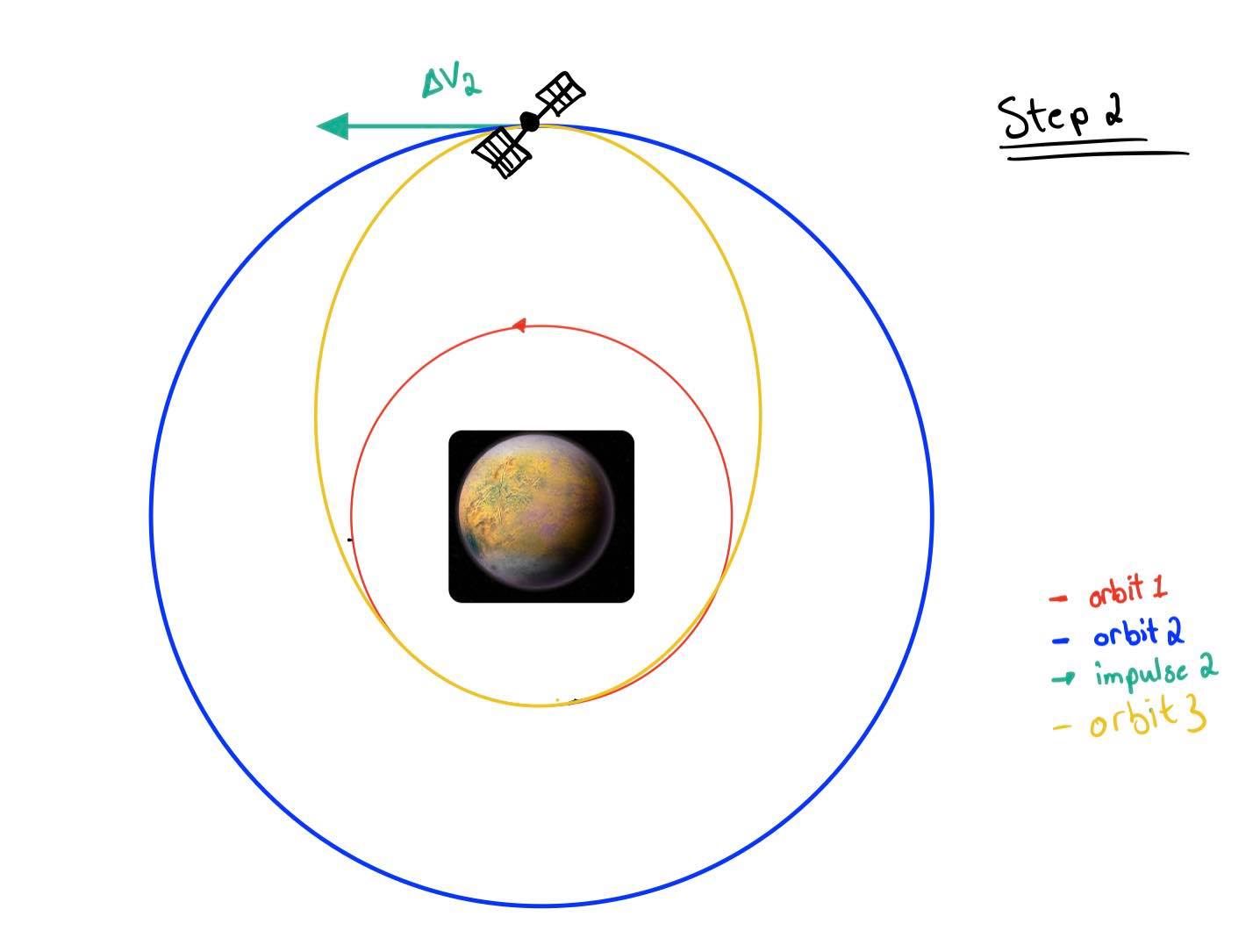
We boost our craft again to enter orbit 2, this time the boost is given by:
\(\Delta v_2=\sqrt{\dfrac{\mu}{r_2}}\left(1- \dfrac{2r_1}{r_1+r_2} \right)\)
Where \(\mu\) is \(GM\) of the primary body (the sun here), \(r_1\)and \(r_2\) are the radii of the first and the second orbit. \(\Delta v_2\) is the acceleration at the second stage.
Have I told you of the Limner sacrifice? It is where I make a sacrifice to the gods in exchange for help when I'm stuck with a problem I can't solve due to technical or conceptual errors. This is my case now, what the sacrifice is, is something I cannot disclose at the moment, perhaps at a later time I will. I have asked the gods to help me place my satellite in a stable orbit around my destination planet. But I would still like to proceed to explain what I was trying to do. At first I was going to try trial and error until I got the right results, using the plots as my guide. But then I came across Hohmann-transfer which is what I will explain but was unable to actually do.
Trial and error method
Firstly I would find when exactly my planets were closest to each other such that we launch our satellite accordingly.
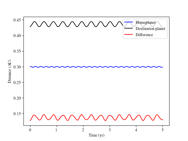
The harmonic oscillating plot of the planets makes sense with what we know of the planetary orbits, that the distance between them and the star oscillates back and forth. The difference plot is also expected to look like this as when you take the difference of two very different functions you get a wobbly function. The important thing is to see when exactly they are closest. A bonus would be if that minimum trough is not exactly sharp but more round, because then we have a longer time at which the planets are quite close to each other giving us a longer time frame that we can operate with, such things help a lot when we're trying trial and error.
The trajectory would have looked different from the Hohmann transfer method.
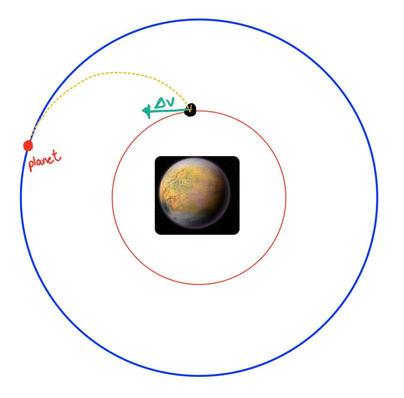
How was I going to use the plots as my guide? Well if the transfer orbit is not in between the home planet's orbit and the destination planet's orbit then we know something's wrong. If the transfer orbit is falling short, as in we're headed in a spiral towards the scorching sun then the velocity is too low. If the transfer orbit is shooting us far far away, then we're using too much fuel and we need to reduce the velocity. Magnitude is not the only problem that can arise, also the direction the velocity is pointed as we might have some sign errors, those are notorious when working with vectors.
For real space probes, there is always unknown systematic errors that are tough to account for, for example the planetary orbits might have some uncertainties, the pull from moons etc. So you would usually have a software that would correct the trajectory by using the orientation software we made last time and finding out how far we have deviated from the original trajectory and then executing a boost to put us back in orbit, such a thing doesn't need to be done too many times but not doing it might mean we miss the planet all together.
The good thing about brute force trial and error is that all that jazz is accounted for because we're actually shooting satellites as experiments. So we don't need a trajectory correcting system.
One more thing to consider before launching is hitting our target, consider the situation where you have a bow and an arrow and you would like to hit a moving target. You would have to release the arrow where the target isn't but rather will be by the time you get there. So here we would calculate the time it took our craft to get where we need it needs to be and then launch accordingly, we would use Figure 7 as a guide as well.
Okay so assuming we did that, and after 30 trials that are just a bit too close or a bit too far, we would aim to be withing this distance away from the target planet. \(l = |\vec r|\sqrt{\dfrac{M_p}{10M_s}}\)
Where r is the distance from the spacecraft to the star, \(M_p\) and \(M_s\) are the masses of the planet and the star respectively.
So what would I do when we're that close? Then I'll calculate what my velocity needs to be such that I stay in a stable circular orbit using the equation we derived last scroll. It's not that simple though, because I would then have to find the unit vector from the planet to my craft, the rotate that vector clockwise or anticlockwise depending on the motion of the circular orbit, rotating the unit vector gives us the tangential velocity's direction which then we multiply by the v_stable to find the required velocity. Knowing the velocity we need and the velocity we have, we can perform a boost or whatever the opposite of boost is called to reach the target velocity and and be in orbit happily ever after.
Normally the results would be here, a large plot with lovely results. This time the results (with the help of the gods) are just two pairs of numbers and time. We have that at t = 1 year, the position of the satellite is (0.38758, -0.193766) AU and our velocity is (3.36902, 8.17901) AU/yr. This is it, the main result, using this velocity and position at the specified time, we would be in stable orbit around our destination planet. I would test these results by plotting it the results on a position graph and see if it orbits the destination planet.
Numerical accuracy is crucial to this part, especially when you're close to an astronomical body. To be safe I would have very high time steps to ensure a good accurate trajectory but not too high as to not spend 3 hours executing the code, one solution to this could be reducing the timesteps when we're coasting freely and increasing it when we're sufficiently close to a heavy astronomical body. Worth noting that increasing the timesteps will improve accuracy. How big an effect does this error have on this part? I think the uncertainties could have been smaller but some amount of uncertainty would be acceptable.
How realistic are the results? Well we can compare it to the ISS. The ISS orbits at a height of 408 km, and our satellite is at a height 100 km. The speed that ISS orbits with is 1.6 AU/yr, meanwhile our velocity is around 8.8 AU/yr. Not too bad given the amount of assumptions and all. Also the velocity required to stay in a stable orbit is smaller the farther away we are (remember the expression for v stable). I give this result the stamp of approval.
Assumptions in this part:
- The spacecraft is allowed to freely adjust its angular orientation without the use of fuel. This is a good assumption because the fuel needed to rotate a spacecraft is not very large, a small injection from the back of the spacecraft is enough to spin it around a bit, not taking it into consideration makes the calculations a bit easier.
-
The duration of a boost is incredibly insignificant compared to the duration of the entire journey. We may therefore regard them as instantaneous. Although it obviously takes some time for the spacecraft to accelerate to the velocity of the new orbit, this assumption is reasonable when the burn time of the rocket
is much smaller than the period of the orbit - I ignored relativistic effects. We (or any other body) is nowhere near the speed of light for it to have any effect
- I assumed that all orbits exist in the same xy-plane. I ignored the z-axis.
- I ignored all other astronomical bodies but this has no effect on our trial and error method of doing things, otherwise we would have to correct the trajectories.