Modelling our atmosphere

We're going to model the atmosphere.

Again, I'm doing brief introduction, mainly focusing only on solving the problem and analyzing the results, not much explaining will be done here.

We want to take measurements and get closer to our planet but without actually entering the atmosphere, no one likes air resistance. So we'll drop low, we can use the the radius of earth and the definition of low orbit, make a factor out of it and find then the corresponding low destination planet orbit.

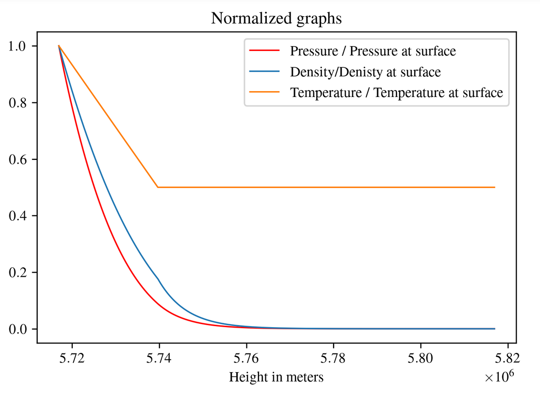
Low earth orbit is a little less than one third of the earth's radius, and it's defined using the orbital period being less than a specific number (11 orbits per day if I remember correctly). We'll use that logic and push it a bit farther. One third of our destination's planet's radius is 1905.644 km above surface. So we have to be lower than that, exactly how much we'll come back to after, looking at density of air will provide us with some useful insight. But how will we reduce our height? We know that the radius of the orbit is determined by the kinetic energy of the body in orbit (we get this from the conservation of mechanical energy). So all we have to do is reduce kinetic energy and the easiest way to do that is by reducing our velocity. With this way we can just boost a tiny bit in the direction opposite to our velocity vector, and see what happens. We don't need to be as close as possible, so it's not worth risking, we have sensors on the craft that sense when the air resistance has a non-negligible effect, which then we can start over again and not brake that much. Another way one can go as low as possible, is to look at where the density of the air is <1% of the density on the surface, now we'll actually model the density next.

_______________________________________________


We calculated the mean molecular weight using this formula

\(\mu = \frac{1}{m_p}\sum ^N_{i=1} l_i \cdot m_i\)

where mp is the mass of a proton (or approximately that of a hydrogen atom), N is the total number of gasses we have, l is the percentage that gas i makes up in the atmosphere, mi is the mass of the N molecules. This way we get an average of the molecules we're working with. More discussion of this will be presented at the end of this scroll.

Inserting the numbers in we get 27.3, the number has no units because we divide AMU by AMU (atomic mass unit). What does this result mean? We have to discuss a bit. For every single point on our atmosphere where there are gasses we have average atomic weight of 27.3, which means every point is comprised of 25% of each point.

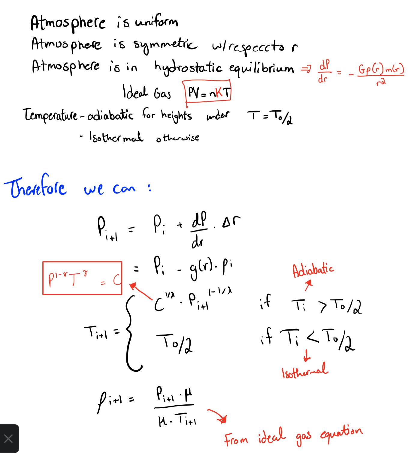
Alright so we have some equations here that we put together to make an algorithm, here's how it looks:
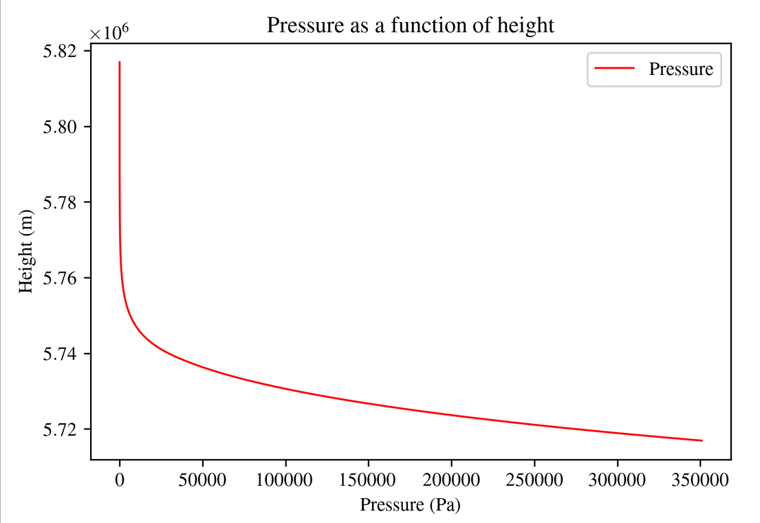
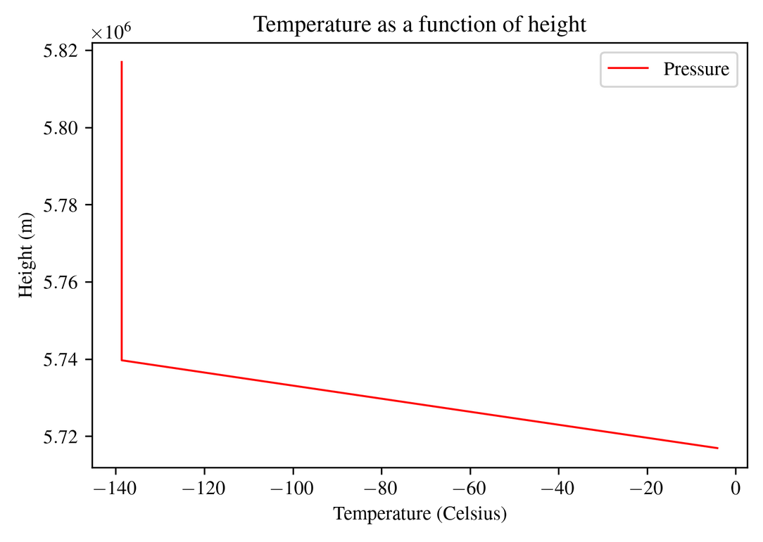
Bildet kan inneholde: håndskrift, gjøre, linje, skråningen, parallell.
Calculations and assumptions that allow us to make an algorithm
Running this algorithm yields the following juice:
 
Temperature plotted in Celsius instead of Kelvin.
 
 
Now before we analyze and discuss the results, let's look at a normalized graph, which can give us some insight. Note that we haven't included any captions but included the information needed in the plot title.


The graphs all go down as we expect them to. The reason being that the air gets thinner as we increase altitude (even on earth), and using the ideal gas equation we see that when you reduce the density, the temperature and the pressure decreases. It's not all that simple though, there are many more factors but it sort of boils down to this.
 
The main result

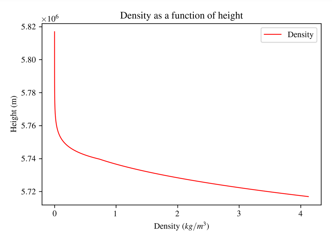
Now that we have modeled very important factors of the atmosphere, we can then interpolate the data points and even extrapolate them (extrapolating is when you find values that are outside of your dataset while interpolating is finding values that are within and between your datasets.). This way we have a density profile that allows us to know what to expect in terms of air resistance as a function of height above the planet. To make sure the interpolate function worked I simply plotted the original plot and the interpolated function plot to make sure they're more or less accurate.

Are my results consistent and realistic?

Our initial temperature has its own unrealistic and bad assumptions made, which we have calculated in another scroll. However, if the initial temperature is more or less correct then we good. Let's look compare our values to earth and see if it's even close

Table comparing Earth to Our Destination Planet
  Destination Planet Planet Earth

Surface air density \(kg/m^3\)

4.12 1.225
Surface air pressure (Pa) 350 000 100 000
Surface air temperature (\(^\circ C \)) -4 15


This is great, we are in the same order of magnitude! We can't look much beyond orders of magnitude as earth's atmosphere is incredibly complex and these numbers are just averages computed in massively different ways. We even see higher density and higher pressure which link up well together.
 
There are quite a few things that can lead to errors and uncertainties. First are the assumptions, one of them is that or every single point on our atmosphere where there are gasses we have average atomic weight of 27.3, which means every point is comprised of 25% of each gas. Now that is a bold assumption to make, here's why: If we look at the earth we see for example that in the troposphere (0-15 km) we have 99% of all water in the whole atmosphere of earth, above that we have again almost all the ozone. This can be made better by having a complex atmospheric profile where for each "region" we have a distribution different from the one we're running.
 
Another error source is the usual steps that we use in the integration algorithm, we must balance between time to run programs and accuracy, and from there determine what is fine and what is not. In our case we used steps of 0.5 meter which is not too little but could be increased to ensure accuracy, however I would like to point out that it wouldn't make a huge difference as there are no big changes in the derivative \(dP/dr\) throughout the height that would force us to have smaller steps to resolve the details.
 
Another assumptions and error sources are for example assuming spherical symmetry, p = p(r), as in the density around the planet in one spherical shell is exactly the same allover that shell with radius r. That is quite unrealistic, we can look at the earth as an example and the values you get around and above the poles is very different from the values around and above the equator. One more thing is that we carry on the uncertainty from last scroll, namely not knowing exactly which gasses we have, however the effect on the average will not be too vast.
 
Having said all that, I think our results not exactly accurate, and not very realistic but we have to make do with what we've got, and that's exactly what we'll do, come join us to scout for landing sites.
 
_____________________________________________________________________
 
One more thing we have to get fixed before landing is finding landing spots. We have cameras so we can look at the planet and try to find some nice ground to land on.

BREAKING NEWS: We have some firsthand footage of the surface of the destination planet (SOUND ON).


This last part of the video is the spot we would like to land on. At 4200 seconds, position (-2115878.09372153,-5460707.04873506, 0) meters, I can see my landing site. So to find where it is on the surface of the planet I will find the unit vector of the position vector and multiply it with the radius of the planet. This means we have the position of the landing site at 4200s. We can then use our function that evolves the coordinates to find that spot again after some time. We could try to find more landing sites but it's mostly cloudy for me apart from this beautiful plot of land.
 
Now that we have the coordinate, how do we know where it will be 10 minutes later? I mean the planet spins so we have to somehow account for the time and the spin. How do we achieve this? We switch to spherical coordinates where the spin of the planet only affects one coordinate, then possibly switch back, exactly how? Well that's just basic trigonometry that I'm sure you're good at, but to aid your intelligence let's look at this figure and the accompanying equations.
Bildet kan inneholde: gjøre, skråningen, parallell, sirkel, mønster.
Figure illustrating both Cartesian coordinates and Spherical coordinates. To the right we have equations illustrating how to switch from Cartesian coordinates to spherical coordinates, these relations can be derives using basic trigonometric identities of sin, cos and tan.
So I made a function that returns the coordinates after some time has elapsed. It's a simple function that takes in Cartesian coordinates, switches them to spherical where the spin/angular velocity only affects one parameter in the coordinates, and then after taking the spin after some time into account and getting new spherical coordinates, we switch them back to Cartesian using other relations.
 
Publisert 13. nov. 2021 15:11 - Sist endret 13. nov. 2021 15:11