"Round and around and around and around we go" - Rihanna, 2012
Previously we did simulate a rocket launch, but we couldn't really see anything?? Just some numbers and words confirming it worked or not. Not fun!
What if I told you, we can actually have a look at our solar system by simulating it on our computer?! Then we can pretend we are in space floating around like astronauts.
Let's start simulati-
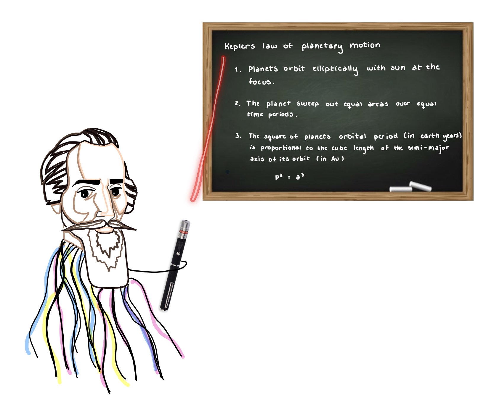
Karl: Bro, you gotta at least introduce them to Kepler.
*knock knock*
Rebecca: Right, we can't simulate orbital motion without him. Come in, Johannes Kepler!!
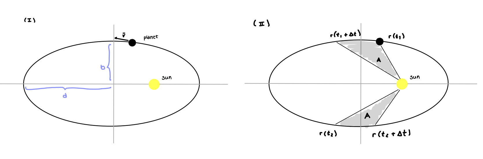
Figure 2.1: Kepler's law of planetary motion presented by J(elly) Kepler Figure 2.2: Kepler's first and second law illustrated
Kepler's first law describes the shape of the orbits as ellipses. It is derived from the observation of variation in velocity, related to Kepler's second law (I will describe this variation in velocity further down). This allows us to use the analytical solution for elliptic orbits (Kepler said it so it must be true, right?) in order to visualise orbits in our solar system, Camphor: \(r(f) = \frac{a(1 - e^2)}{1 + e\cos{f}}\)
where eccentricity, \(e = \sqrt{1 - \frac{b^2}{a^2}}\)
(You may remember the equation for ellipse as, \(\frac{x^2}{a^2}+\frac{y^2}{b^2} =1\) . That is the equation in cartesian coordinates. However, the equation above, \(r(f)\),is in polar coordinates. They are the same, just in different coordinate systems!)
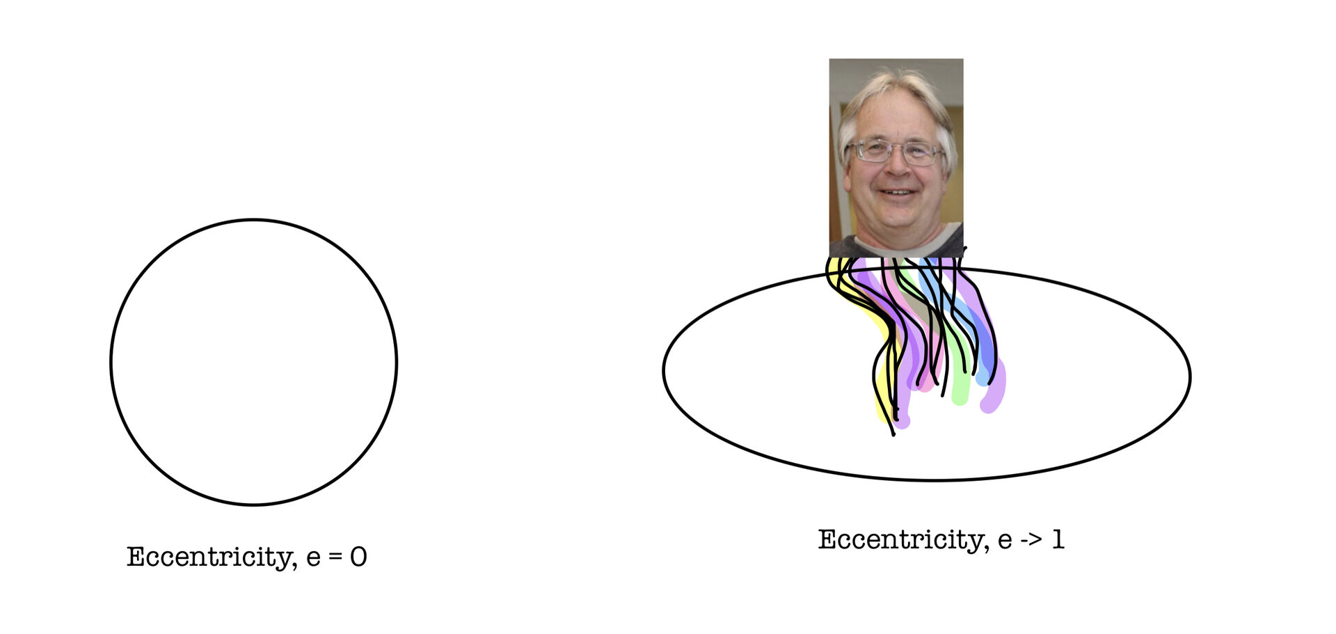
Eccentricity is defined using the ratio between b (semi-minor axis) and a (semi- major axis) for every orbit, check drawing number 1 on figure 2.2 above if you are not sure which axis is which. When the ratio between these two are equal, \(e = 0\), we have a circular orbital shape. When
\(a > b, e \rightarrow 1\), giving us a more elliptical shape.
"A ellipse is just a circle someone sat on" - Tom Lindstrøm1
Figure 2.3: We have nice round circle with eccentricity = 0. If Tom Lindstrøm sat on the circle the semi-major axis gets squished, making it longer than the semi- minor axis and an eccentricity closer to 1. We now have a ellipse, tada!
Kepler's second states the area A swept out during time interval dt is constant. Meaning equal area is swept out for equal lengths of time. This brings us to the fact that the planet must orbit faster near the sun in order to sweep the same area when it is further away, the velocity variation.
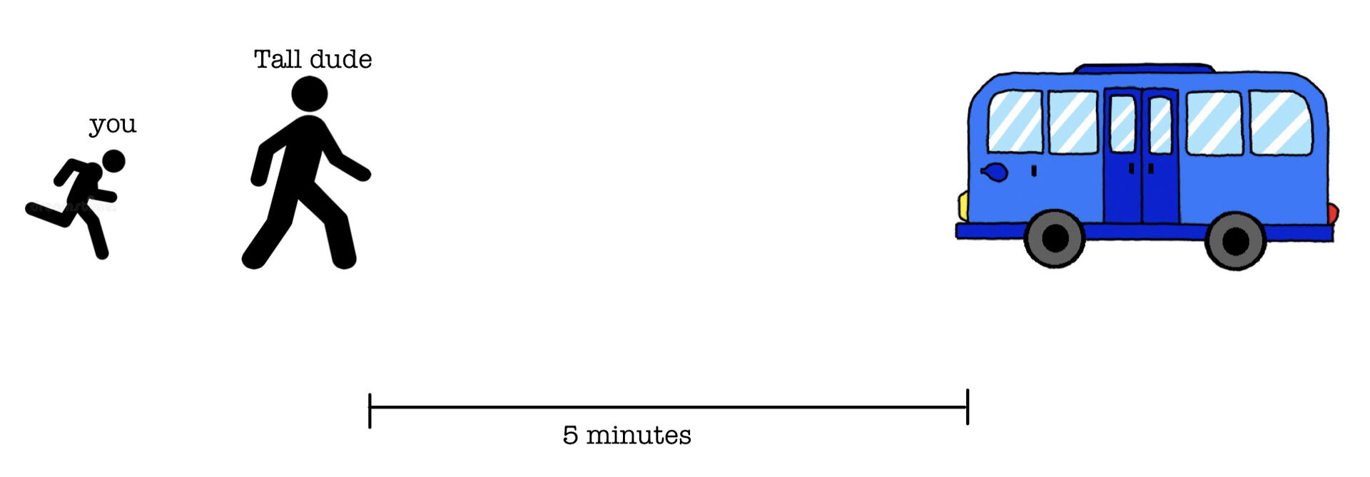
Look at the velocity variation like this. You are a short person of only 150 cm and have to catch a bus that leaves in only 5 minutes. Next to you is a guy of 200 cm with the same goal. Because of his long legs, his steps will get him further compared to you. This means it will take him less time to walk to the bus stop and he will make it perfectly fine. If you want to make it onto the same bus as him, you might want to run or else your short legs wont get you anywhere in time :)
Figure 2.4: Bus scenario
The last law states the relation between the orbital period (in earth years) and the semi- major axis of the orbit, \(P^2 = a^3\). However, this law is WRONG, or not entirely correct. How? Clickhere. We will use the improved version by Newton \(P^2 = \frac{4\pi^2}{\gamma(m_1+m_2)}a^3\)
Fun fact of the day:
Kepler's first law is not entirely correct either, like we thought :)
As described earlier, this is the equation for ellipse, \(r(f) = \frac{p}{1 + e\cos f}\), where \(P = a(1 - e^2)\). For \(0 \leq e < 1\) we have an ellipse.
What if \(e = 1\)? P would then be \(2a\) giving us the equation for parabola!!
Okey, so what if \(e > 1\)? That gives us a \(P = a(e^2 - 1)\), A HYPERBOLA!!
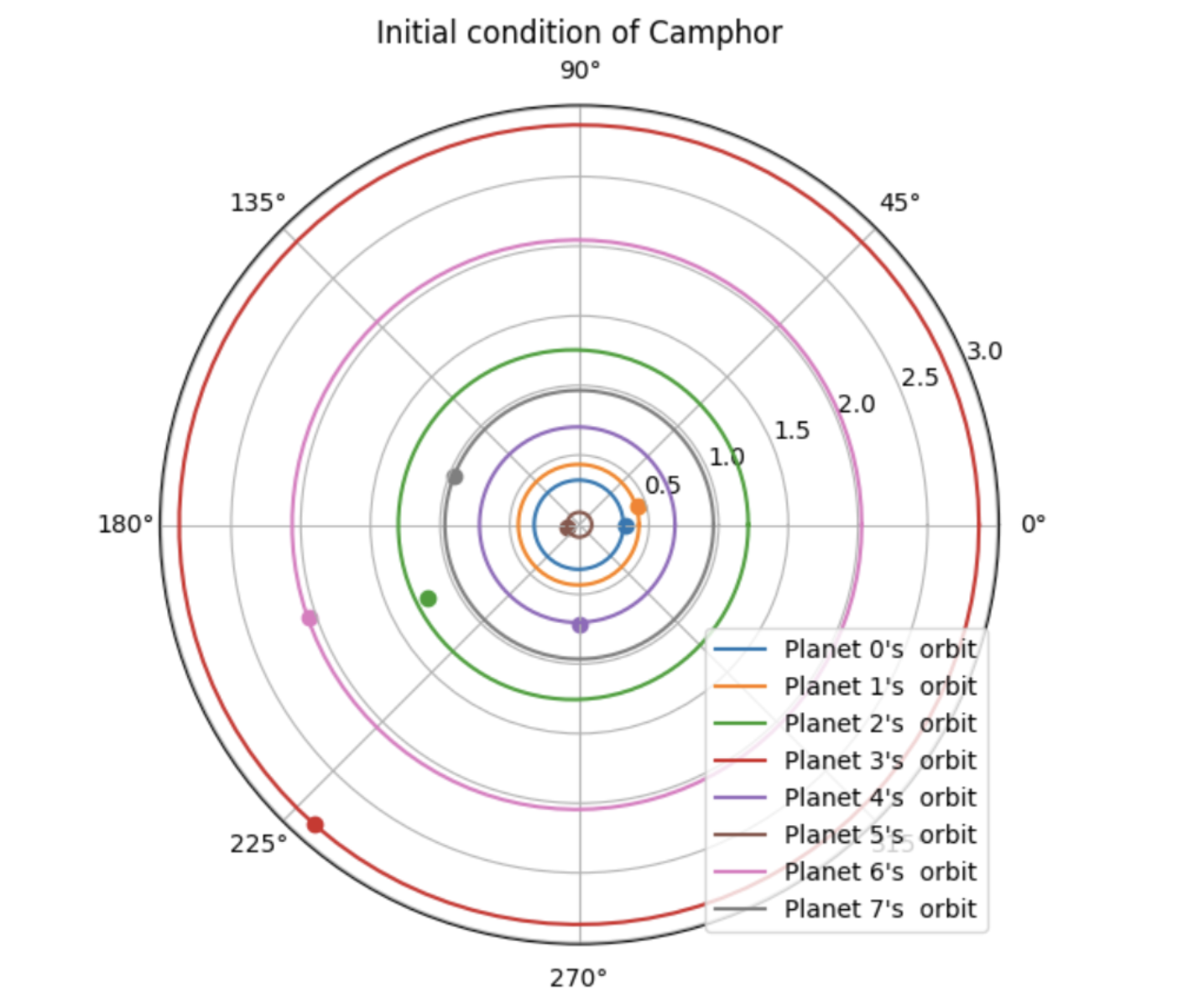
Enough talking, What about a first look at our solar system?. Our wish is to plot orbits in Camphor, in polar coordinates from \([0, 2\pi]\) using the equation for ellipse, \(r(f)\), from Kepler's first law!
(Note! Visualising orbits in polar coordinates does not provide the actual shape of the orbits. These orbits have more of an elliptical shape. Since Kepler provided us with that equation, we shall use it. However, we might switch coordinate system if that benefits us in the future.)
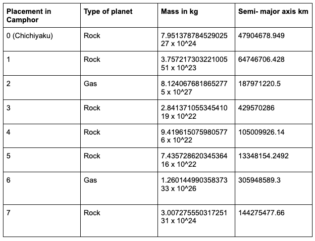
Figure 2.5: Orbits in Camphor. Planet 0 is our home, ChichiyakuFigure 2.6: Information on all of our planets
Look at these beautiful shapes and colors! We even plotted the initial position of every planet. However, this analytical solution does not describe the position of the planets as a function of time. If would be very helpful, it is like having a child. You want to know where your child is at every moment or else it could just run away!
*knock knock*
Rebecca: Oh it's the leap frog to our rescue9!
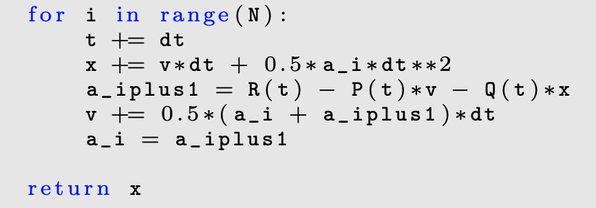
Figure 2.7: The leap frog algorithm from numerical compendium3 that we will be using
The leap frog algorithm will help us numerically simulate planetary motion in Camphor. It is similar to Euler's method we used earlier, but the main difference between these two is leap frog's ability to conserve energy2. This is very useful because planetary motion is actually similar to the motion of oscillating spring. The planet will alternate between moving towards the sun and away from the sun, towards and away. Like a spring bouncing up and down. Acceleration is involved in every time step in the algorithm as we noticed. This benefits us by less information loss since the same information is being used for every loop.
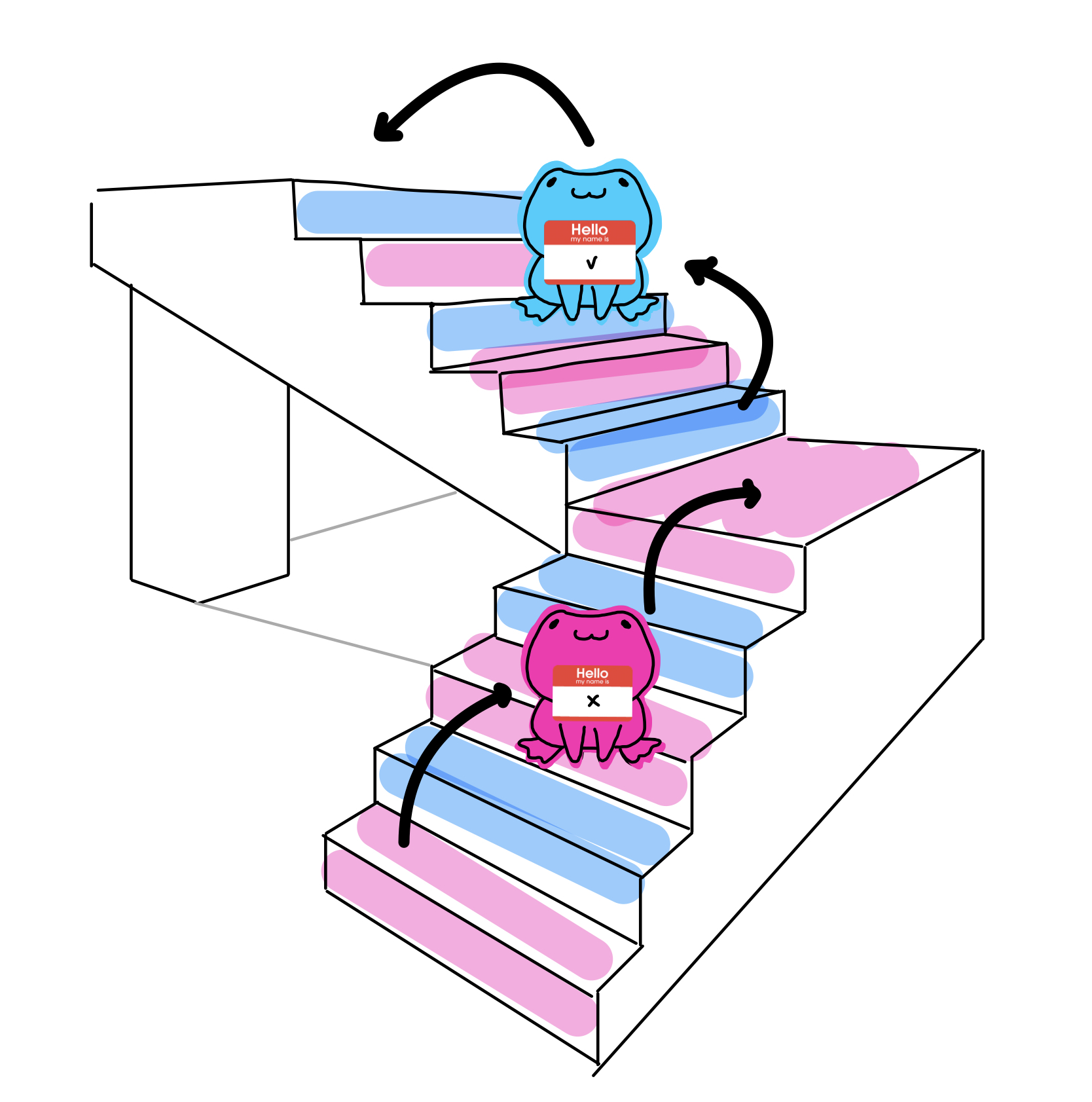
Figure 2.8: The leap frog(gies) helping us. They pick up information from previous stair step and use that to calculate the one they are about to jump onto.
This algorithm reminds me of NASA meetings. You have not heard of it? Ok ok, imagine you are a very clueless student in the course AST2000. You are lucky to have two equally skilled teachers every tuesday. What is better than getting help from only one teacher? GETTING HELP FROM TWO TEACHERS! First teacher Nils can help you, and then teacher Mats Ola can help you, and then they keep switching. So much knowledge and effective, right?
You'll have more information to go on and more knowledge to absorb.
In order for us to use the leap frog, we need to set initial condition for acceleration of the planets. In our simulation we know there is a gravitational force between the sun and our planets and it is the only force describing the acceleration. Like a puzzle we combined this with Newton's second law, and we'll be able to find an expression for acceleration.
(\(m_p\): mass of planet, \(M_{\odot}\): sun mass, \(\vec{r}\): distance vector between sun and planet,
\(\gamma\): gravitational constant, \(\hat{r} \): unit vector of \(\vec{r}\), \(\vec{a}\): acceleration).
With a little algebra and as we norwegians say: with our tongue straight in the mouth, the expression for acceleration of the planets will be \(\vec{a} = \gamma\frac{M_\odot\hat{r}}{r^2} = \gamma\frac{M_\odot\vec{r}}{r^3}\)
Alright alright, enough talking. Time for some leap frog action.
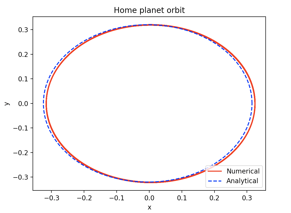
Figure 2.9: Numerical representation of our home planet orbit using leap frog
This time we decided to plot the analytical and numerical orbit in cartesian coordinates to see the shape of both of them on top of each other. There is a small deviation between the analytical and numerical. I have a suspicion it might be because of
1. Numerical errors, which happens when you are approximating and simulating. This is inevitable, it's only a matter of reducing the error.
It is similar to when you are solving a long complicated math equation on a test. You know when you do like a small error in the beginning and it become a consequential error for future calculations? Because you keep using wrong numbers and the more you use the wrong numbers, the worse the error gets and you end up with something totally not correct in the end. Yes, that is how numerical error work except they always have this teeny tiny error from the beginning anyways :)
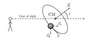
2. The inclination of the orbit is not 90 degrees, meaning it is not parallel to the plane it is visualised in.
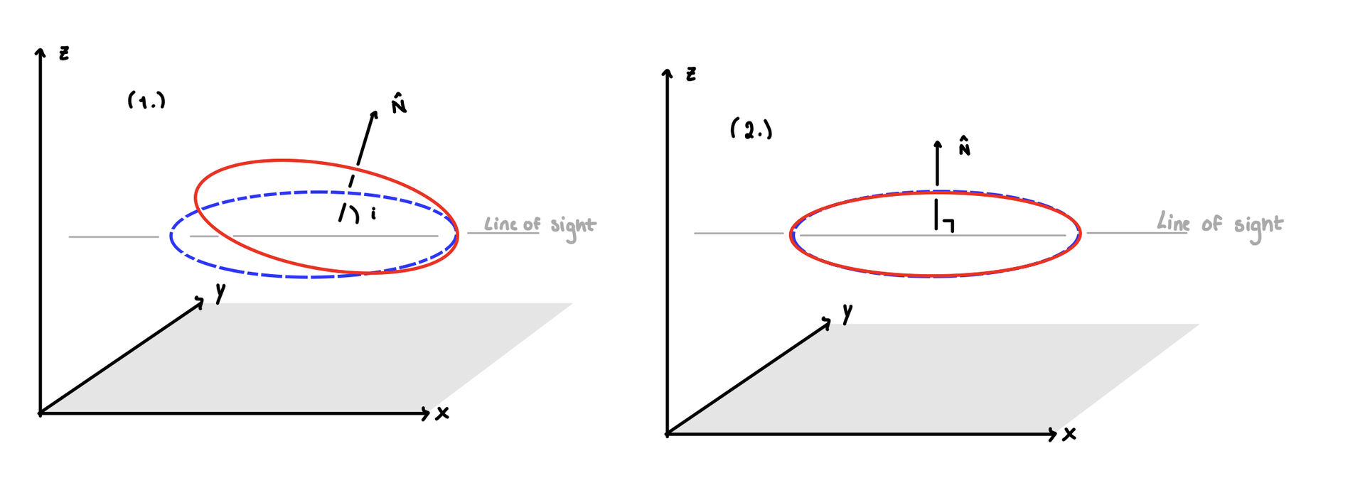
Figure 2.10: Inclination, the angle between line of sight and the normal \(\vec{N}\) to the orbital plane4.Figure 2.11: Situation 1 is how I believe our numerical orbit (red) is placed compared to analytical (blue). Situation 2 is what we want, for them to have the same inclination angle so we can check for accuracy.
Now, you might be wondering: how realistic are these numerical orbits? ... Can we even trust what the computer spit out?