
GOOD EVENING CLASS, TODAY WE'RE TALKING ABOUT NOISE! I'LL JUST HAVE YOU KNOW BEFORE WE START THAT MY EYEJUICE AND EARDRUMS WERE BOTH BLOWN OUT MINUTES BEFORE COMING OUT HERE SO IF YOU HAVE QUESTIONS MAIL THEM TO REBECCA.
I'll just write it down
Noise in the cosmic sence is a whole bunch of different things, from neutrinos, Cosmic radiation, Gravitational waves and Electromagnetic waves, and it's very frustrating to deal with when you're trying to look at something far away in the cosmos, as a huge red disk obscures your microwave-vision.
Essentially we can view noise in a similar way to the background noise in an audio recording, but for the different kinds of waves and particles we can observe in the cosmos. We can begin with a small look at how we'd remove background noise from an audio recording, as the consepts are similar to how we make our obsevations more accurate. When we do an audio recording we'll start off my recording 'nothing', the goal of this is to see what background noise looks like. Once we know this, we can install programmes to nullify the specific sounds creating this background noise, and removing then in order to achieve actual silence. If we take a similar example from radio telescopes; they will fire a lazer beam, of which the wavelength is known, into the atmosphere. When this laser bounces back it will read differenty, but since we know the wavelength we're doing something similar to listening to the background noise in the audio example. Since we now know the disturbances in the atmosphere, we can then adjust for this in the telescopes, and get better observations.
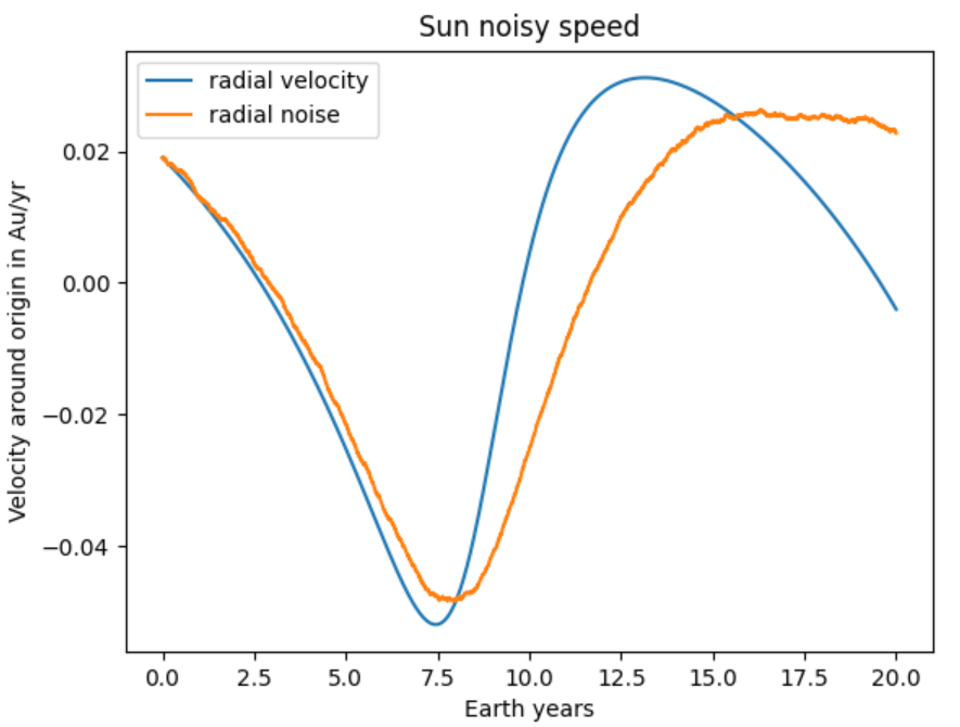
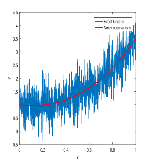
So what's the big deal with this? Well, the picture to the left shows us a curve of the actual measured radial velocity of a star, and an attempt at a noise deviation, of course an actual noise deviation will look slightly different. Which you see in the picture bellow.
Now this kind of noise can be reduced my the mentioned means above, but we can't filter everything out. So we need a way of fitting graphs to this curve, which is a matter of setting up a bunch of expressions which will approximately fit inside, which you'd have done a lot already. But how do we know which one would be the correct one?
It's not like there's a lack of options. To solve this we make use of two central consepts. The first one of these is the central axis theorem. Which states that complex systems, measured over a long enough time, will be distributed in a gaussian manner. In our case this means we can assume the noise's deviation from the actual measurments will have a gaussian distributian above and bellow the graph. So we then also know there should be about as much deviation above, as bellow the graph, and we can select our previously generated guesses depending on which ones have the least difference between the area the distribution spans above the graph vs the area underneath. In other words the graph will run approximately in the middle of all the noise. Next we'll introduce something known as the method of least squares, which allows us to look at a bunch of datapoints, here our gaussianly distributed errors in velocity, and determine the best fitted graph. \(A = \sum\limits_{t_i}{[v_{model}(t_i) - v_{obs}(t_i)]^2}\) where \(v_{model}\) represents the numerous models of the graph we have from earlier. This method aims to look at the difference between the observed and expected graphs, and the closer A is to 0 the better a guess our model is.
Now we'll look at the probability dencity of deviating from the actual velocity by an amount of \(\delta v\), in a single point. The probability dencity is here looking at a uniform distribution of velocities and looking at the probability of the velocity deviating by a certain amount. Much like the gas in our engine. The formula for this is \(P(\delta v) = \frac{1}{\sqrt{2\pi}\sigma_{noise}} e^{-\frac{1}{2}\frac{\delta v ^2}{\sigma_{noise}^2}}\), where \(\sigma_{noise}\) is the area of the distribution where 68,2% of the deviated velocities will be, two will contain 95,4% and three will contial 99,7%. The probabilities of the velocities being in these areas will be independant, meaning they're not affected by the other outcomes, much like rolling a die. The contrary to this would be drawing cards from a deck, and trying to determine the probability of a color or specific type as you go. Since the amount of both desired and undesired cards vary draw by draw the probability will be dependant on what draw you just made and how many you've made. Now looking at a single point isn't gonna tell us much, jell the deviation from the actual velocity won't even be gaussian!
To acieve this we'll need more points, and this brings us to multiplication of probabilities, more precisely, independant ones. Cause multiplying them is very straight forward, you just plop them othether. Now if we look at \(P(\delta v)\) for every point in our graph we get: \(P = P(\delta v_0)*P(\delta v_1)*...*P(\delta v_n)\) which when multiplied together will give us the expression: \(P = \prod\limits_{i = 1}^{N} \frac{1}{\sigma_{noise\space i}}e ^{-\frac{1}{2}\sum\limits_{i}^{n}(\frac{(v_{obs} - v_{real})^2}{\sigma_{noise\space i}})}\) assuming \(\sigma_{noise\space i}\) doesn't vary, if it does we get \(\chi^2 = \sum\limits_{t_i} \frac{[v_{obs}(t_i) - v_{real}(t_i)]^2}{\sigma_{noise\space i}}\). In case you didn't quite catch that, we're using the method of least squares on the exponent of e in order to get a view of the accuracy of whole graph. what allows us to do this is the aformentioned multiplication of independant probabilities. Now all we need to do is plop our noisy graph into this and we should get back our nice and smooth curve. Alternatively you could try reducing the noise to such an inconsequential level to where you wouldn't need to do much to the data, but this is unrealistic. We didn't touch much on how we found the formulas at the beginning, but it's done by slightly varying both the \(\delta v\) and \(\sigma_{noise}\), however we did not have much time to do this, and as such didn't really bother checking wether the velocity difference or sigma would give us the better result. We mainly based it of our numerical maximum speed of the star, in a couple of measurments. The downside of doing it this way is the star may have a slightly different set of motion from what we expect it to and we get into the inclination shenanigans again. Another downside is we can get some pretty outrageous maximum reading, derailing the whole operation, which should be avoidable by selecting our datasets a bit carefully.
Now that should be all, class; dismissed
Oh my, I think my ride is about to leave without me, gotta fly!